Pileup Reweighting and Pileup Mitigation

Overview

Teaching: 40 min
Exercises: 20 min

Questions

• What is pileup and how does it afffect to jets?

• What is the basic jet quality criteria?

Objectives

• Learn about the pileup mitigation techniques used at CMS.

• Learn about about the basic jet quality criteria.

After following the instructions in the setup (if you have not done it yet) :

cd <YOUR WORKING DIRECTORY>/notebooks/DAS/
source /cvmfs/sft.cern.ch/lcg/views/LCG_104/x86_64-centos7-gcc11-opt/setup.sh
jupyter notebook --no-browser --port=8888 --ip 127.0.0.1

This will open a jupyter notebook tree with various notebooks.

What is pileup?

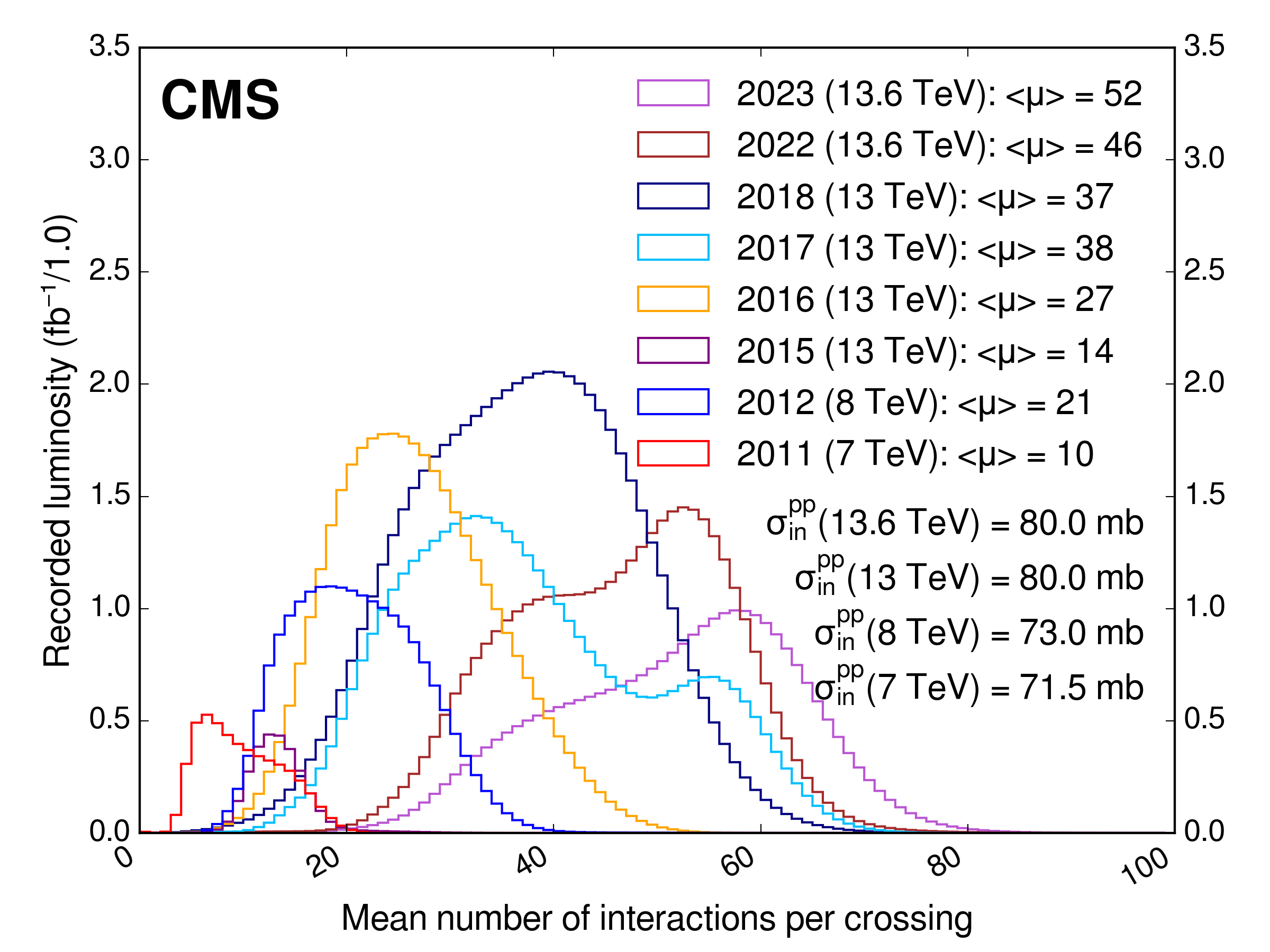
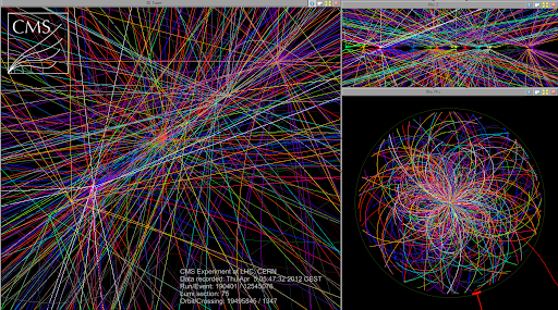
The additional interactions that occur in each bunch crossing because the instantaneous bunch-by-bunch luminosity is very high. Here additional implies that there is a hard-scatter interaction that has caused the event to fire the trigger. The total inelastic cross section is approximately 80mb, so if the luminosity per crossing is of the order 80mb-1 you will get one interaction per crossing, on average.

Types of pileup

We can define two types of pileup:

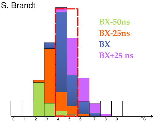
• In-time pileup: the interactions which occur in the bunch crossing that fired the trigger
• Out-of-time pileup: the interactions which occur in the bunch crossings which precede or follow the one which fired the trigger

We need to simulate out-of-time interactions, time structure of detector sensitivity and read-out, and bunch train structure. According to the detector elements used for measuring pileup:

• Tracker: only sensitive to in-time pileup
• Calorimeters: sensitive to out-of-time pileup
• Muon chambers: sensitive to out-of-time pileup

Pileup mitigation algorithms

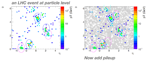
Many clever ways have been devised to remove the effects of pileup from physics analyses and objects. Pileup affects all objects (MET, muons, etc.). We are focusing on jets today.

$\rho$ pileup correction

Imagine making a grid out of your detector, then $\rho$ is the median patch value (pT/area). Therefore, the corrected jet momentum is: \(p_T^{corr} = p_T^{raw} - (\rho \times area)\)

This works because pileup is expected to be isotropic. This is a simplistic version of what the L1 JECs do to remove pileup. More about JECs later.

Exercise 2.1

Before we get into mitigating pileup effects, let’s first examine measures of pileup in more detail. We will discuss event-by-event variables that can be used to characterize the pileup and this will give us some hints into thinking about how to deal with it. We can define:

• NPU: the number of pileup interactions that have been added to the event in the current bunch crossing
• mu: the true mean number of the poisson distribution for this event from which the number of interactions each bunch crossing has been sampled
• $\rho$: rho from all PF Candidates, used e.g. for JECs
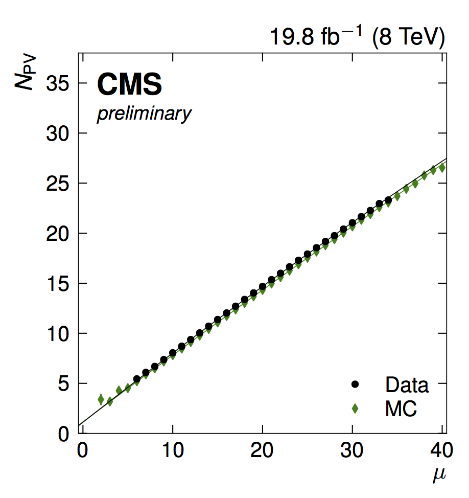
• NPV: total number of reconstructed primary vertices

Open a notebook

For the first part, open the notebook called Pileup.ipynb and run exercise 2.1.

Question 2.1

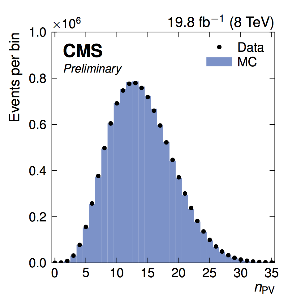
Why are there a different amount of pileup interactions than primary vertices?

Solution 2.1

There is a vertex finding efficiency, which in Run I was about 72%. This means that $N_{PV}\simeq0.72{\cdot}N_{PU}$

Question 2.2

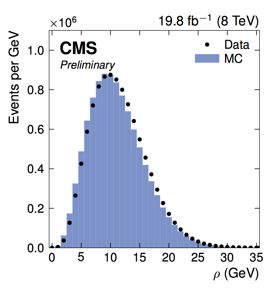
Rho is the measure of the density of the pileup in the event. It’s measured in terms of GeV per unit area. Can you think of ways we can use this information the correct for the effects of pileup?

Solution 2.2

From the jet $p_{T}$ simply subtract off the average amount of pileup expected in a jet of that size. Thus $p_{T}^{corr}{\simeq}p_{T}^{reco}-\rho{\cdot}area$

Question 2.3

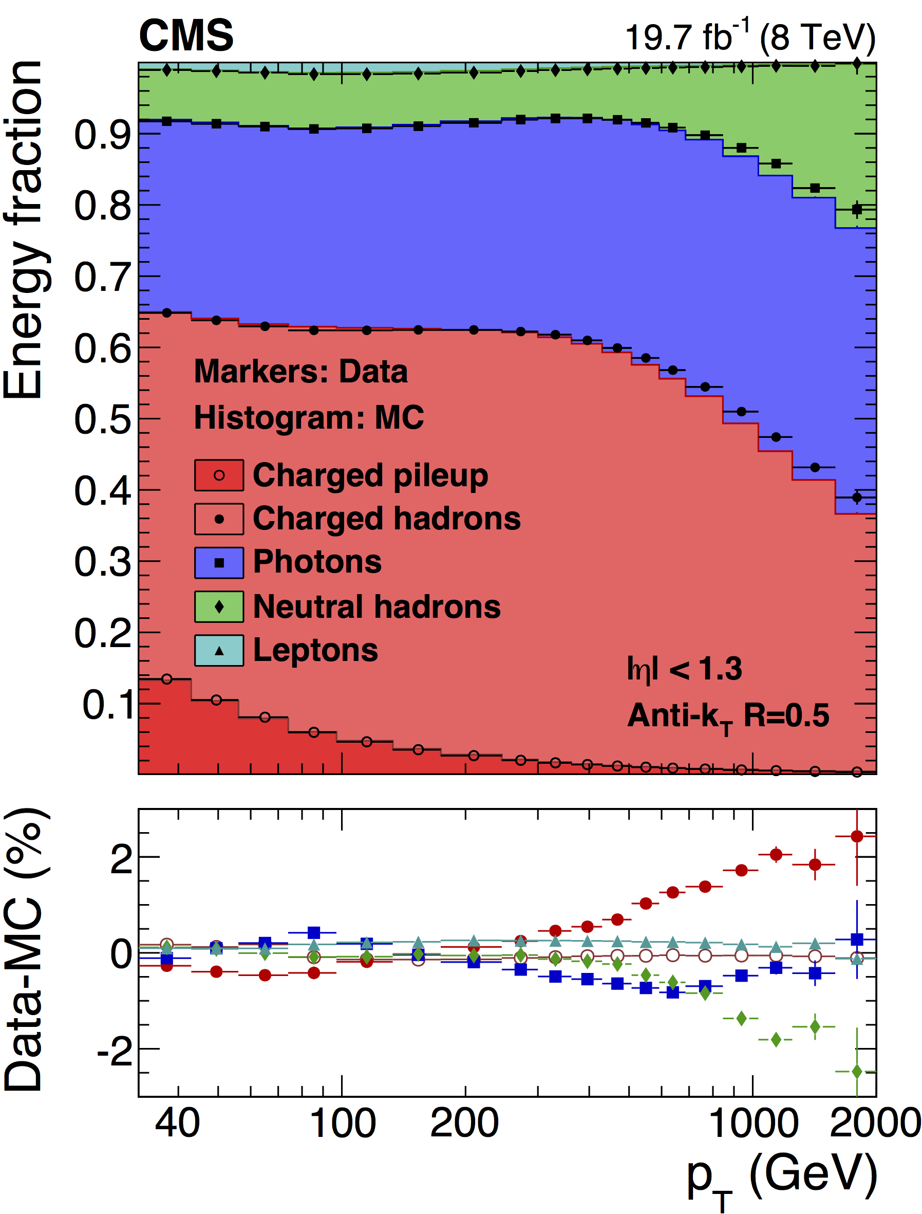
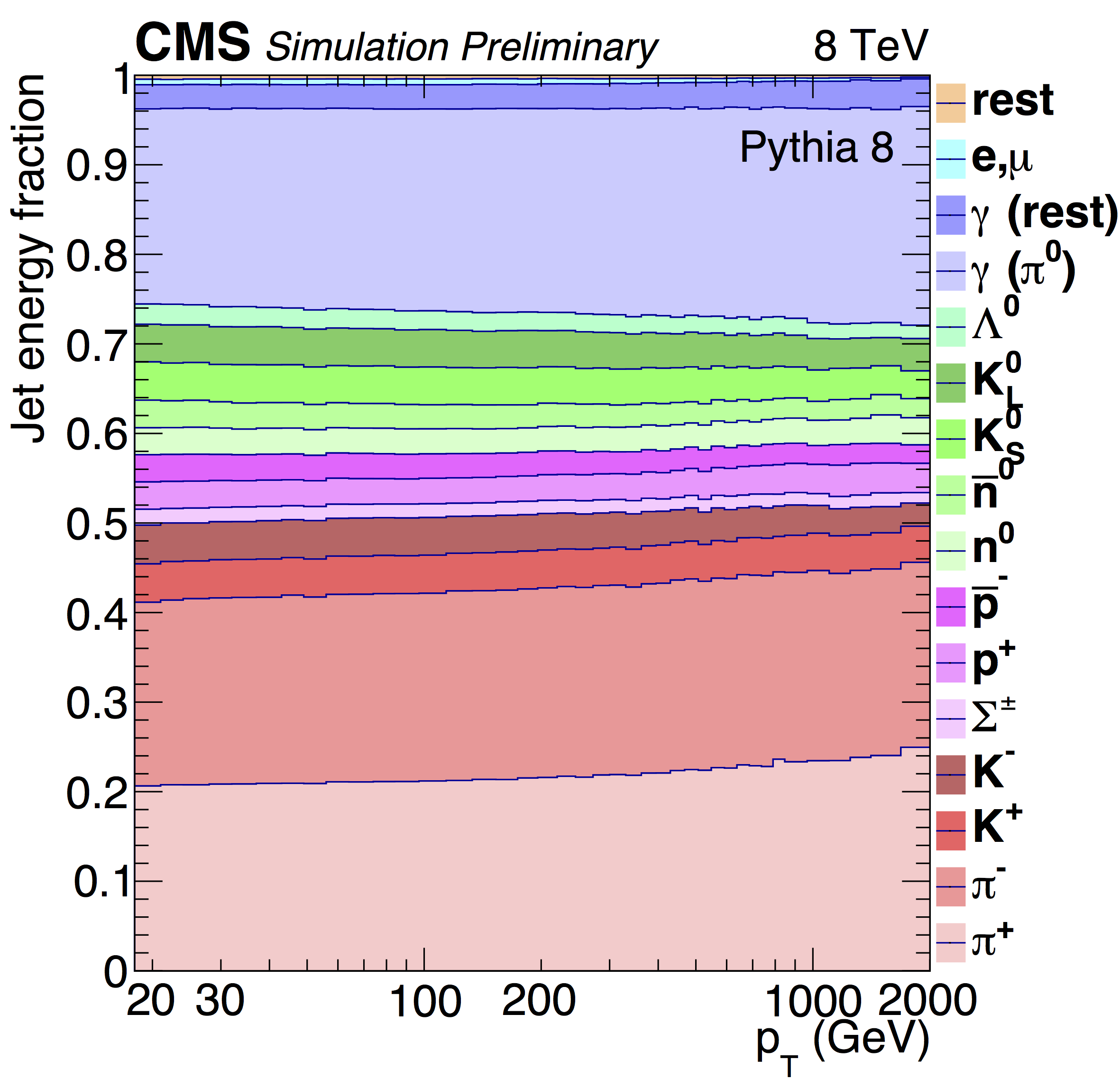
This plot shows the jet composition. Generally, why do we see the mixture of photons, neutral hadrons and charged hadrons that we see?</font>

Solution 2.3

A majority of the constituents in a jet come from pions. Pions come in neutral ($\pi^{0}$) and charged ($\pi^{\pm}$) varieties. Naively you would expect the composition to be two thirds charged hadrons and one third neutral hadrons. However, we know that $\pi^{0}$ decays to two photons, which leads to a large photon fraction.

Charged Hadron Subtraction (CHS)

Tracking is a major tool in CMS. We can identify most charged particles from non-leading primary vertices, CHS removes these particles.

PileUp Per Particle Identification (PUPPI)

Unfortunately, pileup is not really isotropic, it is uneven:

PUPPI is trying to have an inherently local correction based on the following information: A particle from the hard scatter process is likely near (geometrically) other particles from the same interaction and have a generally higher pT. We expect particles from pileup to have no shower structure, have generally lower pT, and be uncorrelated with particles from the leading vertex.

Exercise 2.2

Open a notebook

For this part open the notebook called Pileup.ipynb and run the Exercise 2.2

Discussion 2.1

Do you see any difference in the jet pt for CHS and PUPPI jets? Where you expecting these results?

Pileup reweighting

Start with chosen input distribution – the instantaneous luminosity for a given event is sampled from this distribution to obtain the mean number of interactions in each beam crossing. The number of interactions for each beam crossing that will be part of the event (in- and out-of-time) is taken from a poisson distribution with the predetermined mean. The input distribution is thus smeared by convolving with a poisson distribution in each bin. This is what the observed distribution should look like after the poisson fluctuations of each interaction

The Goal of the pileup reweighting procedure is to match the generated pileup distribution to the one found in data:

• Step 1: Create the weights
• Step 2: Apply the event-by-event weights

Exercise 2.3

Here we are going to produce a file containing the weights used for pileup reweighting using json-pog and correctionlib.

Open a notebook

For this part open the notebook called Pileup.ipynb and run the Exercise 2.3

Question 2.4

Ask yourself what pileup reweighting is doing. How large do you expect the pileup weights to be?

Question 2.5

In what unit will the x-axis be plotted? Another way of asking this is what pileup variable can be measured in both data and MC and is fairly robust?

Solution 2.5

The x-axis is plotted as a function of $\mu$ as this is a true measurement of pileup (additional interactions) and not just some variable which is correlated with pileup. Other options might have been $N_{PV}$, which has an efficiency which is less than 100%, and $\rho$, which assumes that the pileup energy density is uniform. We also get different values of $\rho$ if we measure it for different regions in $\eta$ (i.e. $|\eta|<3$ or $|\eta|<5$).

</details>

Question 2.6

Why do the green and red histograms end arount $\mu\approx38$?

More information

To learn more about pileup, you can follow the CMSDAS short exercise about pileup here: (FIXME)

Noise Jet ID

In order to avoid using fake jets, which can originate from a hot calorimeter cell or electronic read-out box, we need to require some basic quality criteria for jets. These criteria are collectively called “jet ID”. Details on the jet ID for PFJets can be found in the following twiki:

https://twiki.cern.ch/twiki/bin/viewauth/CMS/JetID

The JetMET POG recommends a single jet ID for most physics analysess in CMS, which corresponds to what used to be called the tight Jet ID. Some important observations from the above twiki:

• Jet ID is defined for uncorrected jets only. Never apply jet ID on corrected jets. This means that in your analysis you should apply jet ID first, and then apply JECs on those jets that pass jet ID.
• Jet ID is necessary for most analyses.
• It is complementary to “MET filters” (hit level noise rejection)
• Jet ID is fully efficient (>99%) for real, high-$p_{\mathrm{T}}$ jets used in most physics analysis. Its background rejection power is similarly high.

Exercise 2.4

Open a notebook

For this part open the notebook called Pileup.ipynb and run the Exercise 3.

In nanoAOD is trivial to apply jetID. They are stored as Flags, where events.Jet.jetId>=2 corresponds to tightID and events.Jet.jetId>=6 corresponds to tightLepVetoID.

If you want to know how this flags are stored in nanoAOD, the next block shows the implementation in C++ from a miniAOD file:

Implementation in c++

There are several ways to apply jet ID. In our above exercises, we have run the cuts “on-the-fly” in our python FWLite macro (the first option here). Others are listed for your convenience.

The following examples use somewhat out of date numbers. See the above link to the JetID twiki for the current numbers.

To apply the cuts on pat::Jet (like in miniAOD) in python then you can do :

# Apply jet ID to uncorrected jet
nhf = jet.neutralHadronEnergy() / uncorrJet.E()
nef = jet.neutralEmEnergy() / uncorrJet.E()
chf = jet.chargedHadronEnergy() / uncorrJet.E()
cef = jet.chargedEmEnergy() / uncorrJet.E()
nconstituents = jet.numberOfDaughters()
nch = jet.chargedMultiplicity()
goodJet = \
  nhf < 0.99 and \
  nef < 0.99 and \
  chf > 0.00 and \
  cef < 0.99 and \
  nconstituents > 1 and \
  nch > 0

To apply the cuts on pat::Jet (like in miniAOD) in C++ then you can do:

// Apply jet ID to uncorrected jet
double nhf = jet.neutralHadronEnergy() / uncorrJet.E();
double nef = jet.neutralEmEnergy() / uncorrJet.E();
double chf = jet.chargedHadronEnergy() / uncorrJet.E();
double cef = jet.chargedEmEnergy() / uncorrJet.E();
int nconstituents = jet.numberOfDaughters();
int nch = jet.chargedMultiplicity();
bool goodJet =
  nhf < 0.99 &&
  nef < 0.99 &&
  chf > 0.00 &&
  cef < 0.99 &&
  nconstituents > 1 &&
  nch > 0;

To create selected jets in cmsRun:

from PhysicsTools.SelectorUtils.pfJetIDSelector_cfi import pfJetIDSelector
process.tightPatJetsPFlow = cms.EDFilter("PFJetIDSelectionFunctorFilter",
                                         filterParams = pfJetIDSelector.clone(quality=cms.string("TIGHT")),
                                         src = cms.InputTag("slimmedJets")
                                         )

It is also possible to use the PFJetIDSelectionFunctor C++ selector (actually, either in C++ or python), but this was primarily developed in the days before PF when applying CaloJet ID was not possible very easily. Nevertheless, the functionality of more complicated selection still exists for PFJets, but is almost never used other than the few lines above. If you would still like to use that C++ class, it is documented as an example here.

Question 2.7

What do the jets with jetId represent? Were you expecting more or less jets with jetId==0?

Key Points

• We call pileup to the amount of other processes not coming from the main interaction point. We must mitigates its effects to reduce the amount of noise in our events.

• Many event variables help us to learn how different pileup was during the data taking period, compared to the pileup that we use in our simulations. The pileup reweighting procedure help us to calibrate the pileup profile in our simulations.

• The so-called jetID is the basic jet quality criteria to remove fake jets.