cd <YOUR WORKING DIRECTORY>/notebooks/DAS/
source /cvmfs/sft.cern.ch/lcg/views/LCG_105/x86_64-el9-gcc13-opt/setup.sh
jupyter notebook --no-browser--port=8888 --ip 127.0.0.1
This will open a jupyter notebook tree with various notebooks.
Jet Basics
Jets as signatures of quarks and gluons
Most collisions at hadron colliders involve quarks scattering.
Protons contain quarks and gluons.
Proton collisions are really gluon and quark collisions.
Parton showering → Hadronization → Jet of color neutral particles
Only particles in “color singlet” state are observed in nature, due to color confinement. The kinematic properties of the jet are intended to resemble that of the initial partons. What we try to do wirh our detectors is to measure the decay products to get access to particle/parton level:
After the particles interact with our detector we can reconstruct other stable particles.
What is the composition of jets?
Energy composition: About 65% charged hadrons, 25% neutral pions (photons), 10% neutral hadrons.
What is a jet?
Looking at an event display from our data
How do you determine which particles are included in a jet?
From a list of particles one can form jets, an object to reconstruct the shower of particles produced from a quark or gluon. Each particle belonging to a jet is known as a constituent. Each has a 4-vector that can be used for further studies. This give us a more generalised picture: Almost everything becomes a jet: g/q/t/W/Z/H/PU
We need a method to identify particles which may be the constituents of a jet. This is referred to as a Clustering
Algorithm. A good jet algorithm is infrared and collinear safe. The set of hard jets should be unchanged by soft emission and collinear splitting.
Jet Clustering Algorithms
Most jet algorithms at hadron colliders use a so-called “clustering sequence”. This is essentially a pairwise examination of the input four vectors. If the pair satisfy some criteria, they are merged. The process is repeated until the entire list of particles is exhausted.
These algorithms follow this recipe:
Iteratively find the two particles in the event which are closest in some distance measure and combine them.
Defining \(d_{ij} = min(p^{2p}_{ti},p^{2p}_{tj}) \Delta R^{2}_{ij}/R^2\) and $d_{iB} = p_{ti}^{2p}$. We combine two particles if $d_{ij} < d_{iB}$.
if $p=1$ then kt algorithm (KT)
if $p=0$ then Cambridge Aachen algorithm (CA)
if $p=-1$ then antikt algorithm (AK)
Stop when $d_{ij} > d_{iB}$.
A more visual way of think about the recluster algorithm.
How the different jet algorithms look like in our events?
Comparison of jet areas for four different jet algorithms, from “The anti-kt Clustering Algorithm” by Cacciari, Salam, and Soyez [JHEP04, 063 (2008), arXiv:0802.1189].
Some excellent references about jet algorithms can be found here:
The package used to implement the clustering algorithms in modern colliders is called Fastjet.
This package is used ubiquously in all reconstruction of jets, even though is sometimes hidden in
our reconstruction code. If you want to know more about Fastjet we encourange you to check their
website www.fastjet.fr in your free time.
Jet types at the LHC
Jets are reconstructed physics objects representing the hadronization and fragmentation of quarks and gluons. CMS primarily uses anti-$k_{\mathrm{T}}$ jets with a cone-size of $R=0.4$ to reconstruct this jet type. We have algorithms that distinguish heavy-flavour (b or c) quarks (which are in the domain of the BTV POG), quark- vs gluon-originated jets, and jets from the main $pp$ collision versus jets formed primarily from pileup particles.
However, quarks and gluons are only part of the story! At the LHC, the typical collision energy is much greater than the mass scale of the known SM particles, and hence, even heavier particles like top quarks, W/Z/Higgs bosons, and heavy beyond-the-Standard-Model particles can be produced with large Lorentz boosts. When these particles decay to quarks and gluons, their decay products are collimated and overlap in the detector, making them difficult to reconstruct as individual AK4 jets.
Therefore, LHC analyses use jet algorithms with a large radius parameter to reconstruct these objects, called “large radius” or “fat” jets. CMS uses anti-$k_{\mathrm{T}}$ jets with $R=0.8$ (AK8) as the standard large-radius jet, while ATLAS uses AK10.
You can also read these excellent overviews of jet substructure techniques:
Several ways exist to determine the “area” of the jet over which the input constituents lay. This is very important in correcting pileup, as we will see, because some algorithms tend to “consume” more constituents than others and hence are more susceptible to pileup. Furthermore, the amount of energy inside a jet due to pileup is proportional to the area, so it is essential to know the jet area to correct this effect.
In the first exercise we will compare jet areas for different types of jets.
For this part, open the notebook called Jets_101.ipynb (if it is not opened) and run Exercise 1.1
Discussion 1.1
Before you run the exercise 1.1, what type of
distribution do you expect for the areas of the AK4 and AK8 jets?
Question 1.1
After exercise 1.1: Try modifying the plotting cell to add vertical lines at area values corresponding to $\pi R^2$. Do the histogram peaks line up with these values?
The jet algorithms take as input a set of 4-vectors. At CMS, the most popular jet type is the “Particle Flow Jet,” which attempts to use the entire detector at once and derive single four vectors representing specific particles. For this reason, it is very comparable (ideally) to clustering generator-level four-vectors.
Monte Carlo Generator-level Jets (GenJets)
GenJets are pure Monte Carlo simulated jets. They are helpful for analysis with MC samples. GenJets are formed by clustering the four-momenta of Monte Carlo truth particles. This may include “invisible” particles (muons, neutrinos, WIMPs, etc.).
As no detector effects are involved, the jet response (or jet energy scale) is 1, and the jet resolution is perfect, by definition.
GenJets include information about the 4-vectors of constituent particles, the energy’s hadronic and electromagnetic components, etc.
Calorimeter Jets (CaloJets)
CaloJets are formed from energy deposits in the calorimeters (hadronic and electromagnetic), with no tracking information considered. In the barrel region, a calorimeter tower consists of a single HCAL cell and the associated 5x5 array of ECAL crystals (the HCAL-ECAL association is similar but more complicated in the endcap region). The four-momentum of a tower is assigned from the energy of the tower, assuming zero mass, with the direction corresponding to the tower position from the interaction point.
In CMS, CaloJets are used less often than PFJets. Their use includes performance studies to disentangle tracker and calorimeter effects and trigger-level analyses where the tracker is neglected to reduce the event processing time. ATLAS makes much more use of CaloJets, as their version of particle flow is less mature than CMS’s.
Particle Flow Jets (PFJets)
Particle Flow candidates (PFCandidates) combine information from various detectors to estimate particle properties based on their assigned identities (photon, electron, muon, charged hadron, neutral hadron).
PFJets are created by clustering PFCandidates into jets and contain information about contributions of every particle class: Electromagnetic/hadronic, Charged/neutral, etc.
The jet response is high. The jet pT resolution is good, starting at 15–20% at low pT and asymptotically reaching 5% at high pT.
In CMS we recluster two types of PFJets:
CHS jets = “Charge Hadron Subtracted” jets = remove charged PF particles associated to non-primary vertices (remove charged pileup). These are the default in Run 2.
PUPPI jets = PF constituents have been weighted/removed by an algorithm (PUPPI) which is designed to remove pileup contamination (more info in PU section). These are the default in Run 3.
Full jet and MET reconstruction in CMS
Exercise 1.2
Open a notebook
For this part, open the notebook called Jets_101.ipynb (if it is not opened) and run Exercise 1.2
Question 1.2
After running the notebook’s Exercise 1.2: As you can see, the agreement between Calo, Gen, and Pfjet could be better! Can you guess why?
Solution 1.2
We need to apply the jet energy corrections (JEC) described in the next exercise. But before doing that, we’ll review the jet clustering algorithms used in CMS.
Jet types and algorithms in CMS
The standard jet algorithms are all implemented in the CMS reconstruction software, CMSSW. However, a few algorithms with specific parameters (namely AK4, AK8, and CA15) have become standard tools in CMS; these jet types are extensively studied by the JetMET POG, and are highly recommended. These algorithms are included in the centrally produced CMS samples, at the AOD, miniAOD, and nanoAOD data tiers (note that miniAOD and nanoAOD are most commonly used for analysis, while AOD is much less common these days, and is not widely available on the grid). Other algorithms can be implemented and tested using the JetToolbox (more in the following link).
In this part of the tutorial, you will learn how to access the jet collection included in the CMS datasets, compare the different jet types, and create your own collections.
AOD
This twiki summarizes the respective labels by which each jet collection can be retrieved from the event record for general AOD files. This format is currently used for specialized studies, but you can use the other formats for most analyses.
MiniAOD
Three main jet collections are stored in the MiniAOD format, as described here.
slimmedJets: are AK4 energy-corrected jets using charged hadron subtraction (CHS) as the pileup removal algorithm. Jets are selected with $p_T >10$ GeV (typically analysis cut will be at least pT>20). This is the default jet collection for CMS analyses for Run II. In this collection, you can find the following jet algorithms, as well as other jet-related quantities:
b-tagging
Pileup jet ID
Quark/gluon likelihood info embedded.
slimmedJetsPUPPI: are AK4 energy-corrected jets using the PUPPI algorithm for pileup removal. This collection will be the default for Run III analyses.
slimmedJetsAK8: ak4 AK8 energy-corrected jets using the PUPPI algorithm for pileup removal. Jets are selected iwth pT >170 GeV with all information, including PF candidate links(typically analysis cut will be at least pT>200). This has been the default collection for boosted jets in Run II. In this collection, you can find the following jet algorithms, as well as other jet-related quantities:
Softdrop mass
n-subjettiness and energy correlation variables
Access to softdrop subjets with pT >30 GeV: minimal information for 3 leading jets.
Access to the associated AK8 CHS jet four-momentum, including soft drop and pruned mass, and n-subjectness.
Examples of how to access jet collections in miniAOD samples
Below are two examples of how to access jet collections from these samples. This exercise does not intend for you to modify code in order to access these collections, but rather for you to look at the code and get an idea about how you could access this information if needed.
In C++
Please take a look at the file jmedas_miniAODAnalyzer.C with your favourite code viewer.
You can run this code by using the python config file jmedas_miniAODtest.py from your terminal once you have set a CMSSW environment and download this JMEDAS package. This script will only print out some information about the jets in that sample. Again, the most important part of this exercise is to get familiar with how to access jet collections from miniAOD. Take a good look at the prints this script produces to your terminal. Use a new directory outside the cloned JMEDAS directory.
cmsrel CMSSW_14_0_7
cd CMSSW_14_0_7/src
cmsenv
mkdir Analysis
cd Analysis
ln-s <PATH_TO_JMEDAS_DIRECTORY> JMEDAS
scram b
cmsRun $CMSSW_BASE/src/Analysis/JMEDAS/scripts/jmedas_miniAODtest.py
In Python
Now take a look at the file jmedas_miniAODtest_purePython.py.
This code can be run with simple python in your terminal. Similar as in the case for C++, the output of this job is some information about jets. The most important part of the exercise is to get familiar with how to access jet collections using python from miniAOD.
NanoAOD is a “flat tree” format, meaning you can access the information directly with simple ROOT or even simple Python tools (like numpy or pandas). This format is recommended for analyses in CMS, unless one needs to access other variables not stored in nanoAOD. This tutorial will only use nanoAOD files.
In nanoAOD, only AK4 CHS jets ( Jet ) and AK8 PUPPI jets ( FatJet ) are stored in Run 2. For Run 3, AK4 and AK8 jets are PUPPI jets. The jets in nanoAOD are similar to those in miniAOD, but not identical (for example, the $p_{\mathrm{T}}$ cuts might be different). In short:
Jet = ak4PFJetsCHS
pT >15 GeV
Similar to miniAOD content, but many more (up-to-date) quantities (e.g. JEC)
FatJet = ak8PFJetsPUPPI
Similar content to miniAOD, but many more (up-to-date) quantities such as DeepXXX taggers
A full set of variables for each jet collection can be found in this website.
Also possible to customize nanoAOD. JME/BTV have their extended format with more jet collections and/or PF candidates. It is a common format for “automatised” workflows and ML training.
Note
There are several advanced tools on the market which allow you to do sophisticated analysis using nanoAOD format, including RDataFrame, NanoAOD-tools, or Coffea. We encourage you to look at them and use the one you like the most. However, we are going to use coffea for this tutorial.
Jet properties
A short list of jet properties that we can find in nanoAOD are:
Jet 4-vector = sum of all constituent particle 4-vectors: energy, pT, η, Φ
Jet constituent fractions, ex. charged hadron energy fraction
Jet area = area in η-Φ plane in which an infinitely soft particle will be clustered with the jet
Jet tagging information
and many more
Exercise 1.3
Open a notebook
This preliminary exercise will illustrate some of the basic properties of jets, like the four-momentum quantities: pt, eta, phi, and mass. We will use nanoAOD files currently widely used with the CMS Collaborators. For more information about nanoAOD follow this link. At the end of the notebook, you will be able to see all the quantities stored in the Jet collection.
For this part, open the notebook called Jets_101.ipynb and run Exercise 1.3
Discussion 1.2
Have you seen these jet quantities before? Were you expecting something different?
Discussion 1.3
Did you plot other jet quantities stored in nanoAOD? Do you understand the meaning of them?
Key Points
Jet is a physical object representing hadronic showers interacting with our detectors. A jet is usually associated with the physical representation of quark and gluons, but they can be more than that depending of their origin and the algorithm used to define them.
A jet is defined by its reclustering algorithm and its constituents. In current experiments, jets are reclusted using the anti-kt algorithm. Depending on their constituents, in CMS, we called jets reclustered from genparticles as GenJets, calorimeter clusters as CaloJets, and particle flow candidates as PFJets.
Pileup Reweighting and Pileup Mitigation
Overview
Teaching: 40 min
Exercises: 20 min
Questions
What is pileup and how does it afffect to jets?
What is the basic jet quality criteria?
Objectives
Learn about the pileup mitigation techniques used at CMS.
Learn about about the basic jet quality criteria.
After following the instructions in the setup (if you have not done it yet) :
If using LXPLUS:
cd <YOUR WORKING DIRECTORY>/notebooks/DAS/
source /cvmfs/sft.cern.ch/lcg/views/LCG_105/x86_64-el9-gcc13-opt/setup.sh
jupyter notebook --no-browser--port=8888 --ip 127.0.0.1
This will open a jupyter notebook tree with various notebooks.
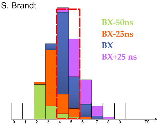
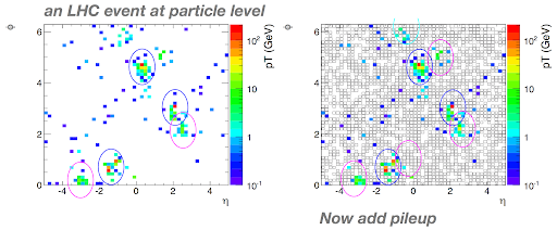
What is pileup?
Pileup are the additional interactions that occur in each bunch crossing because
the instantaneous bunch-by-bunch luminosity is very high.
Here additional implies that there is a hard-scatter interaction that has caused
the event to fire the trigger. The total inelastic cross section is approximately 80mb, so if the luminosity per crossing is of the order 80mb-1 you will get one interaction per crossing, on average.
Types of pileup
We can define two types of pileup:
In-time pileup: the interactions which occur in the bunch crossing that fired the trigger
Out-of-time pileup: the interactions which occur in the bunch crossings which precede or follow the one which fired the trigger
We need to simulate out-of-time interactions, time structure of detector sensitivity and read-out, and bunch train structure. According to the detector elements used for measuring pileup:
Tracker: only sensitive to in-time pileup
Calorimeters: sensitive to out-of-time pileup
Muon chambers: sensitive to out-of-time pileup
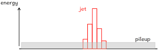
Pileup mitigation algorithms
Many clever ways have been devised to remove the effects of pileup from physics analyses and
objects. Pileup affects all objects (MET, muons, etc.). We are focusing on jets today.
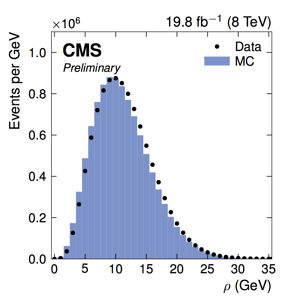
$\rho$ pileup correction
Imagine making a grid out of your detector, then $\rho$ is the median patch value (pT/area). Therefore, the corrected jet momentum is:
\(p_T^{corr} = p_T^{raw} - (\rho \times area)\)
This works because pileup is expected to be isotropic. This is a simplistic version of what the L1 JECs do to remove pileup. More about JECs later.
Exercise 2.1
Before we get into mitigating pileup effects, let’s first examine measures of pileup in more detail. We will discuss event-by-event variables that can be used to characterize the pileup and this will give us some hints into thinking about how to deal with it. We can define:
NPU: the number of pileup interactions that have been added to the event in the current bunch crossing
mu: the true mean number of the poisson distribution for this event from which the number of interactions each bunch crossing has been sampled
$\rho$: rho from all PF Candidates, used e.g. for JECs
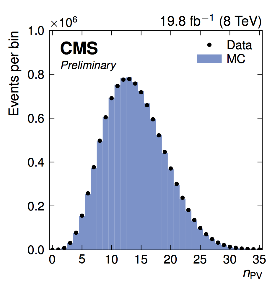
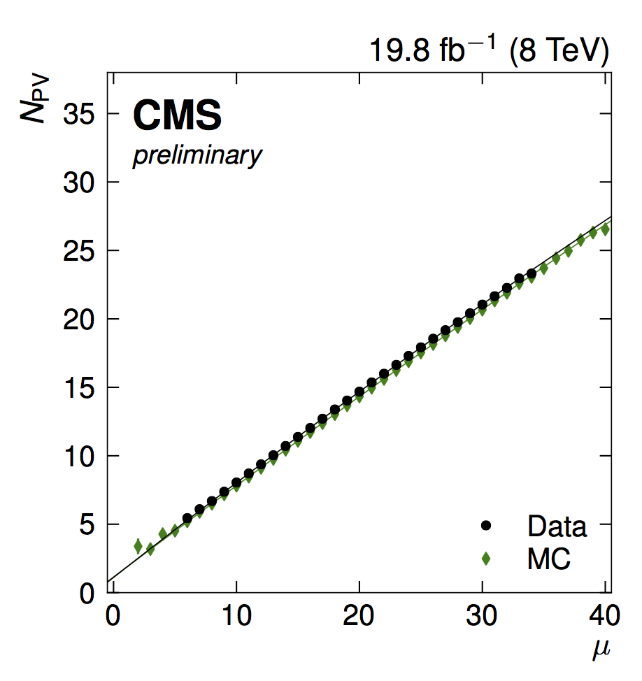
NPV: total number of reconstructed primary vertices
Open a notebook
For the first part, open the notebook called Pileup.ipynb and run exercise 2.1.
Question 2.1
Why are there a different amount of pileup interactions than primary vertices?
Solution 2.1
There is a vertex finding efficiency, which in Run I was about 72%. This means that $N_{PV}\simeq0.72{\cdot}N_{PU}$
Question 2.2
Rho is the measure of the density of the pileup in the event. It’s measured in terms of GeV per unit area. Can you think of ways we can use this information the correct for the effects of pileup?
Solution 2.2
From the jet $p_{T}$ simply subtract off the average amount of pileup expected in a jet of that size. Thus $p_{T}^{corr}{\simeq}p_{T}^{reco}-\rho{\cdot}area$
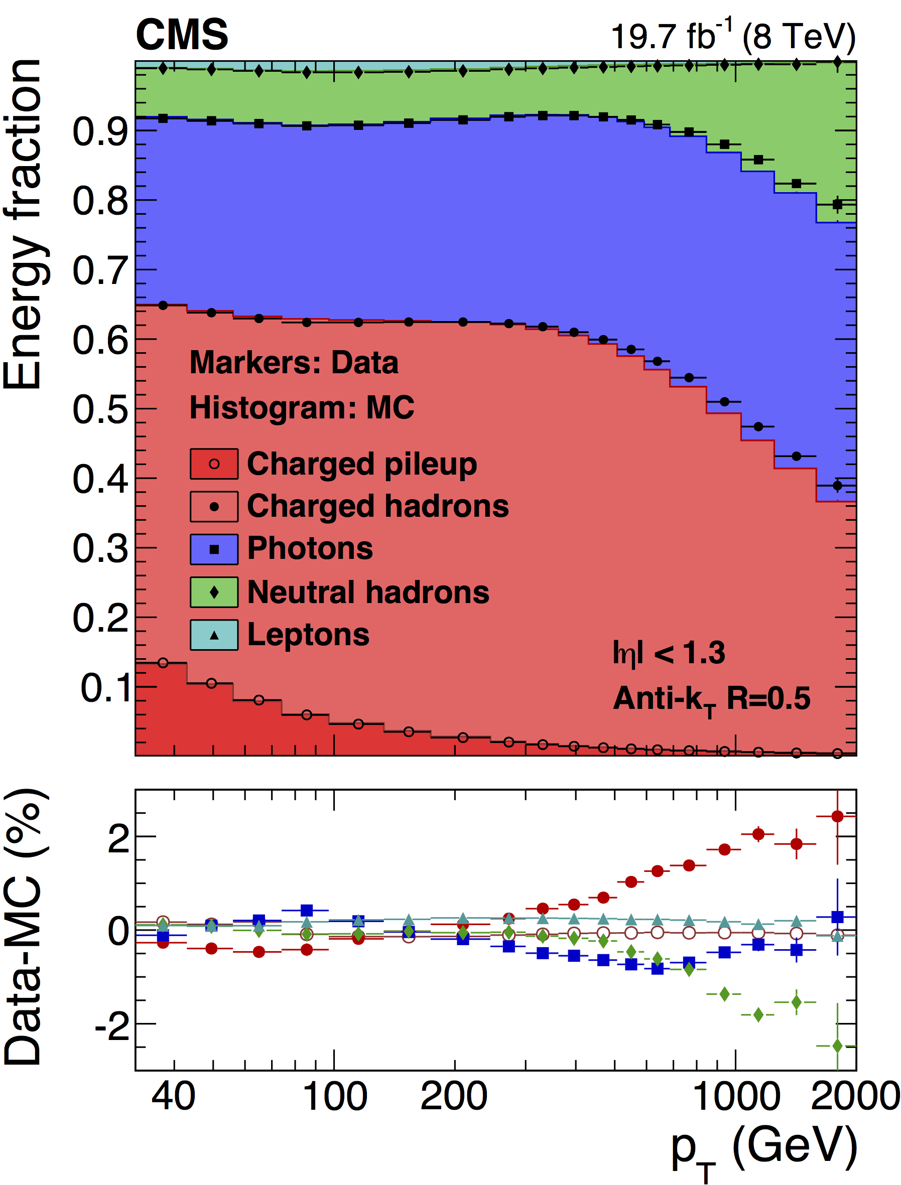
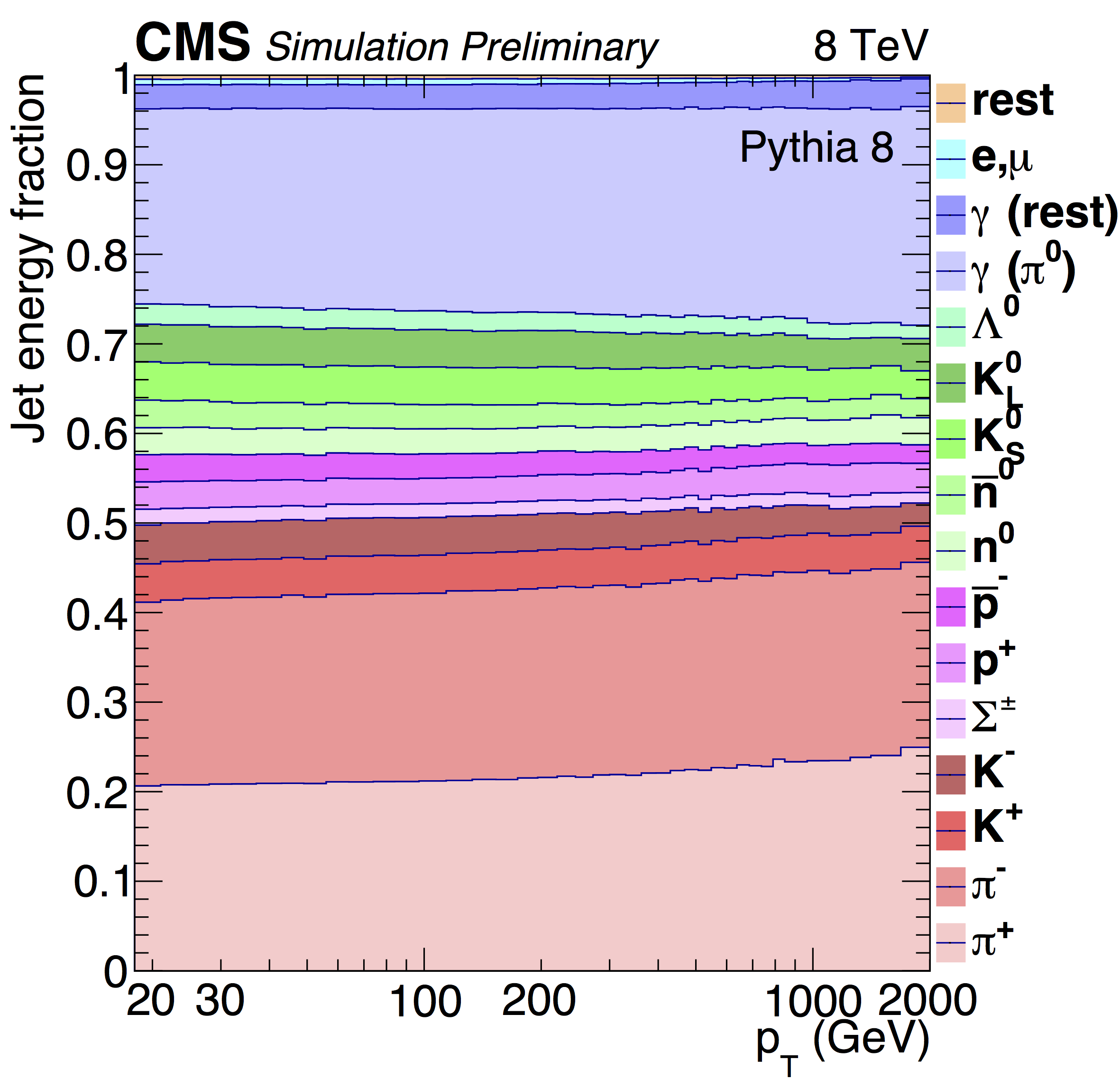
Question 2.3
This plot shows the jet composition. Generally, why do we see the mixture of photons, neutral hadrons and charged hadrons that we see?</font>
Solution 2.3
A majority of the constituents in a jet come from pions. Pions come in neutral ($\pi^{0}$) and charged ($\pi^{\pm}$) varieties. Naively you would expect the composition to be two thirds charged hadrons and one third neutral hadrons. However, we know that $\pi^{0}$ decays to two photons, which leads to a large photon fraction.
Charged Hadron Subtraction (CHS)
Tracking is a major tool in CMS. We can identify most charged particles from non-leading primary vertices, CHS removes these particles.
PileUp Per Particle Identification (PUPPI)
Unfortunately, pileup is not really isotropic, it is uneven:
PUPPI is trying to have an inherently local correction based on the following information: A particle from the hard scatter process is likely near (geometrically) other particles from the same interaction and have a generally higher pT. We expect particles from pileup to have no shower structure, have generally lower pT, and be uncorrelated with particles from the leading vertex.
Exercise 2.2
Open a notebook
For this part open the notebook called Pileup.ipynb and run the Exercise 2.2
Discussion 2.1
Do you see any difference in the jet pt for CHS and PUPPI jets? Where you expecting these results?
Pileup reweighting
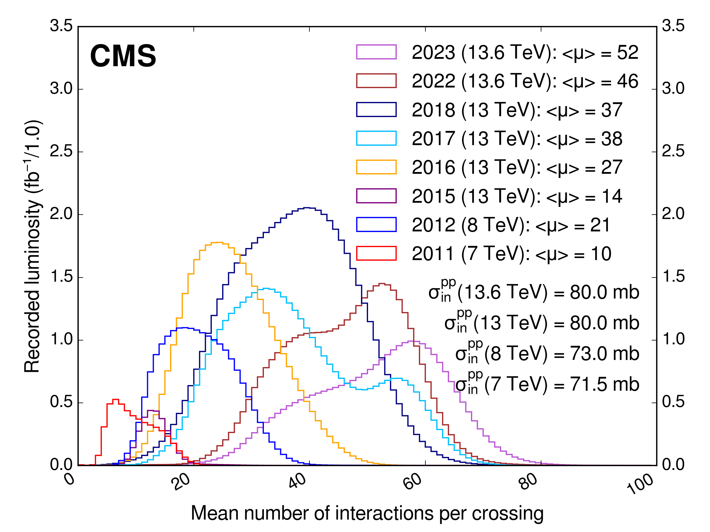
Start with chosen input distribution – the instantaneous luminosity for a given event is sampled from this distribution to obtain the mean number of interactions in each beam crossing. The number of interactions for each beam crossing that will be part of the event (in- and out-of-time) is taken from a poisson distribution with the predetermined mean. The input distribution is thus smeared by convolving with a poisson distribution in each bin. This is what the observed distribution should look like after the poisson fluctuations of each interaction
The Goal of the pileup reweighting procedure is to match the generated pileup distribution to the one found in data:
Step 1: Create the weights
Step 2: Apply the event-by-event weights
Exercise 2.3
Here we are going to produce a file containing the weights used for pileup reweighting using
json-pog and correctionlib.
Open a notebook
For this part open the notebook called Pileup.ipynb and run the Exercise 2.3
Question 2.4
Ask yourself what pileup reweighting is doing. How large do you expect the pileup weights to be?
Question 2.5
In what unit will the x-axis be plotted? Another way of asking this is what pileup variable can be measured in both data and MC and is fairly robust?
Solution 2.5
The x-axis is plotted as a function of $\mu$ as this is a true measurement of pileup (additional interactions) and not just some variable which is correlated with pileup. Other options might have been $N_{PV}$, which has an efficiency which is less than 100%, and $\rho$, which assumes that the pileup energy density is uniform. We also get different values of $\rho$ if we measure it for different regions in $\eta$ (i.e. $|\eta|<3$ or $|\eta|<5$).
</details>
Noise Jet ID
In order to avoid using fake jets, which can originate from a hot calorimeter cell or electronic read-out box, we need to require some basic quality criteria for jets. These criteria are collectively called “jet ID”. Details on the jet ID for PFJets can be found in the following twiki:
The JetMET POG recommends a single jet ID for most physics analysess in CMS, which corresponds to what used to be called the tight Jet ID. Some important observations from the above twiki:
Jet ID is defined for uncorrected jets only. Never apply jet ID on corrected jets. This means that in your analysis you should apply jet ID first, and then apply JECs on those jets that pass jet ID.
Jet ID is necessary for most analyses.
It is complementary to “MET filters” (hit level noise rejection)
Jet ID is fully efficient (>99%) for real, high-$p_{\mathrm{T}}$ jets used in most physics analysis. Its background rejection power is similarly high.
Exercise 2.4
Open a notebook
For this part open the notebook called Pileup.ipynb and run the Exercise 3.
In nanoAOD is trivial to apply jetID. They are stored as Flags, where events.Jet.jetId>=2 corresponds to tightID and events.Jet.jetId>=6 corresponds to tightLepVetoID.
If you want to know how this flags are stored in nanoAOD, the next block shows the implementation in
C++ from a miniAOD file:
Implementation in c++
There are several ways to apply jet ID. In our above exercises, we have run the cuts “on-the-fly” in our python FWLite macro (the first option here). Others are listed for your convenience.
The following examples use somewhat out of date numbers. See the above link to the JetID twiki for the current numbers.
To apply the cuts on pat::Jet (like in miniAOD) in python then you can do :
# Apply jet ID to uncorrected jet
nhf = jet.neutralHadronEnergy() / uncorrJet.E()
nef = jet.neutralEmEnergy() / uncorrJet.E()
chf = jet.chargedHadronEnergy() / uncorrJet.E()
cef = jet.chargedEmEnergy() / uncorrJet.E()
nconstituents = jet.numberOfDaughters()
nch = jet.chargedMultiplicity()
goodJet = \
  nhf < 0.99 and \
  nef < 0.99 and \
  chf > 0.00 and \
  cef < 0.99 and \
  nconstituents > 1 and \
  nch > 0
To apply the cuts on pat::Jet (like in miniAOD) in C++ then you can do:
It is also possible to use the PFJetIDSelectionFunctor C++ selector (actually, either in C++ or python), but this was primarily developed in the days before PF when applying CaloJet ID was not possible very easily. Nevertheless, the functionality of more complicated selection still exists for PFJets, but is almost never used other than the few lines above. If you would still like to use that C++ class, it is documented as an example here.
Question 2.7
What do the jets with jetId represent? Were you expecting more or less jets with jetId==0?
Key Points
We call pileup to the amount of other processes not coming from the main interaction point. We must mitigates its effects to reduce the amount of noise in our events.
Many event variables help us to learn how different pileup was during the data taking period, compared to the pileup that we use in our simulations. The pileup reweighting procedure help us to calibrate the pileup profile in our simulations.
The so-called jetID is the basic jet quality criteria to remove fake jets.
Jet energy corrections and resolution
Overview
Teaching: 40 min
Exercises: 20 min
Questions
What are jet energy correction?
What is jet energy resolution?
Objectives
Learn about how we calibrate jets in CMS.
Learn about the resolution of the jets and its effect.
After following the instructions in the setup (if you have not done it yet) :
cd <YOUR WORKING DIRECTORY>/notebooks/DAS/
source /cvmfs/sft.cern.ch/lcg/views/LCG_105/x86_64-el9-gcc13-opt/setup.sh
jupyter notebook --no-browser--port=8888 --ip 127.0.0.1
This will open a jupyter notebook tree with various notebooks.
Jet Energy Corrections
Let’s define the jet pt response $R$ as the ratio between the measured and the true pt of a jet
from simulation. We expect that the average response is different from 1 because of pileup adding
energy or non-linear calorimeter response.
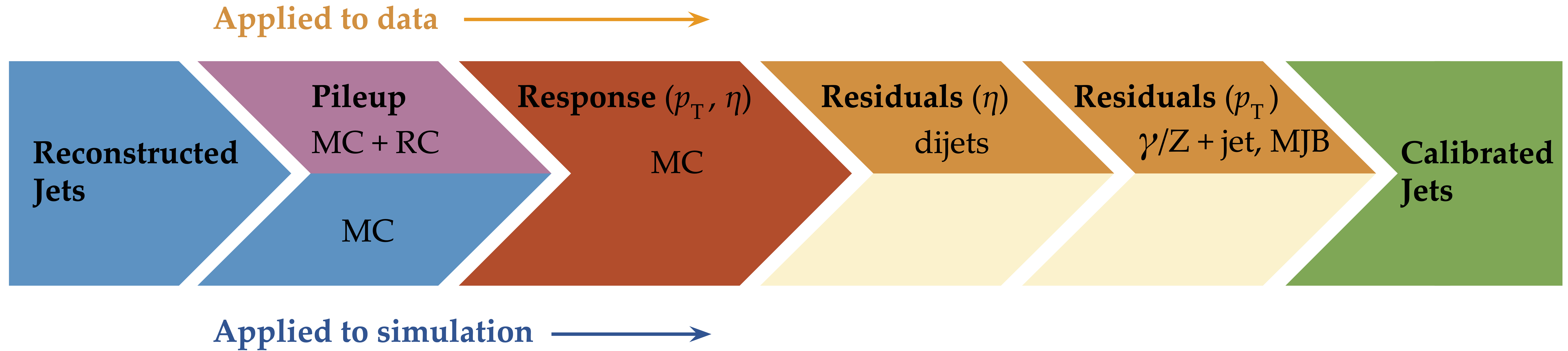
Jet energy corrections (JEC) corrects reconstructed jets (on average) back to particle level.
This is done against many useful metrics, like $p_T^{gen}$, $\eta$, area, pileup. CMS uses a
factorized approach to JECs:
Pileup corrections to correct for offset energy (noPU vs. PU jet matching). This is usually called L1FastJet.
Correction to particle level jet vs. 𝑝𝑇 and η from simulation. This is called L2Relative and L3Absolute, or L2L3 together.
Only for data: Small residual corrections (Pileup/relative and absolute) to correct for differences between data and simulation. This is called L2L3Residuals.
Jet energy scale determination in data
Reminder for PUPPI jets
PUPPI jets do not need the L1 Pileup corrections. Starting with Run 3, PUPPI jets are the primary jet collection.
Exercise 3.1
Open a notebook
For this part open the notebook called Jet_Energy_Corrections.ipynb and run the Exercise 3.1
Discussion 1.1
After running Exercise 1 of the notebook, were you expecting differences between these two
distributions? Do you think the differences are large or small?
After running the Exercise 1 of the notebook, we can notice that the
$p_{\mathrm{T}}$ distributions disagree quite a bit between the
GenJets and PFJets.
We need to apply the jet energy corrections (JECs),
a sequence of corrections that address non-uniform responses in
$p_{\mathrm{T}}$ and $\eta$, as well as an average correction for pileup.
The JECs are often updated fairly late in the analysis cycle,
simply due to the fact that the JEC experts start deriving the JECs
at the same time the analyzers start developing their analyses.
For this reason, it is imperative for analyzers to maintain
flexibility in the JEC, and the software reflects this.
For more information and technical details on the jet energy
scale calibration in CMS, look at the following link:
https://cms-jerc.web.cern.ch/JEC/.
It is possible to run the JEC software “on the fly” after you’ve done
your heavy processing (Ntuple creation, skimming, etc).
We will now show one example on how this is done using the latest
correctionlib package and the JME json-pog in the Exercise 2.
json-pog and correctionlib
Currently CMS and the JME POG are supporting the use of the so-called json-pog with the
correctionlib python package, in a way to make the implementation of corrections more uniform.
Specifically, JECs were delivered in the past in a zip file containing txt files where the users could
find the corrections. The json-pog makes this process more generic between CMS POGs, and
correctionlib makes the implementation of this corrections also more generic.
where the string Summer19UL18_V5_MC_L1L2L3Res_AK4PFchs contains the JME nomenclature for
labeling the JECs. In this example:
Summer19UL18_V5_MC corresponds to the JECs campaing; including data processing campaign, JEC version, and if is MC or DATA.
L1L2L3Res is the JEC type. In this case corresponds to the set of L1FastJet, L2Relative, L2L3Residual, L3Absolute
AK4PFchs is the type of jet: ak4 pfjet using CHS as a pileup removal algorithm.
Discussion 1.2
After running Exercise 2 of the notebook, how big is the difference in $p_{\mathrm{T}}$ for corrected and
uncorrected jets? Do you think it is larger at low or high $p_{\mathrm{T}}$?
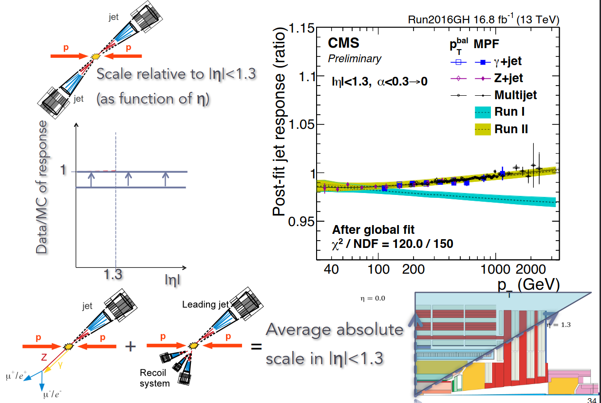
Discussion 1.3
Why do we need to calibrate jet energy? Why is “jet response” not equal to 1? Can you think of a physics process in nature that can help us calibrate the jet response to 1?
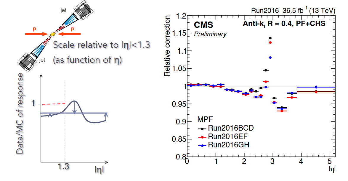
Discussion 1.4
The amount of material in front of the CMS calorimeter varies by $\eta$. Therefore, the calorimeter response to jet is also a function of jet $\eta$. Can you think of a physics process in nature that can help us calibrate the jet response in $\eta$ to be uniform ?
JEC Uncertainties
Since we’ve applied the JEC corrections to the distributions, we should also assign a systematic uncertainty to the procedure. The procedure is explained in this link, and this is part of the Exercise 2.3 of the notebook.
Exercise 3.2
Open a notebook
For this part open the notebook called Jet_Energy_Corrections.ipynb and run the Exercise 3.
Question 1.1
After running the Exercise 3 of the notebook, does the result make sense? Is the nominal histogram always between the up and down variations, and should it be?
Jet Energy Resolution
Jets are stochastic objects.
The content of jets fluctuates quite a lot,
and the content also depends on what actually caused the jet
(uds quarks, gluons, etc).
In addition, there are experimental limitations to the measurement of jets.
Both of these aspects limit the accuracy to which we can measure the
4-momentum of a jet.
The way to quantify our accuracy of measuring jet energy is called the jet
energy resolution (JER). If you have a group of single pions that have the
same energy, the energy measured by CMS will not be exactly the same every
time, but will typically follow a (roughly) Gaussian distribution with a mean
and a width.
The mean is corrected using the jet energy corrections.
It is impossible to “correct” for all resolution effects on a jet-by-jet
basis, although regression techniques can account for many effects.
As such, there will always be some experimental and theoretical uncertainty
in the jet energy measurement, and this is seen as non-zero jet energy resolution.
There is also other jet-related resolutions such as jet angular resolution
and jet mass resolution, but JER is what we most often have to deal with.
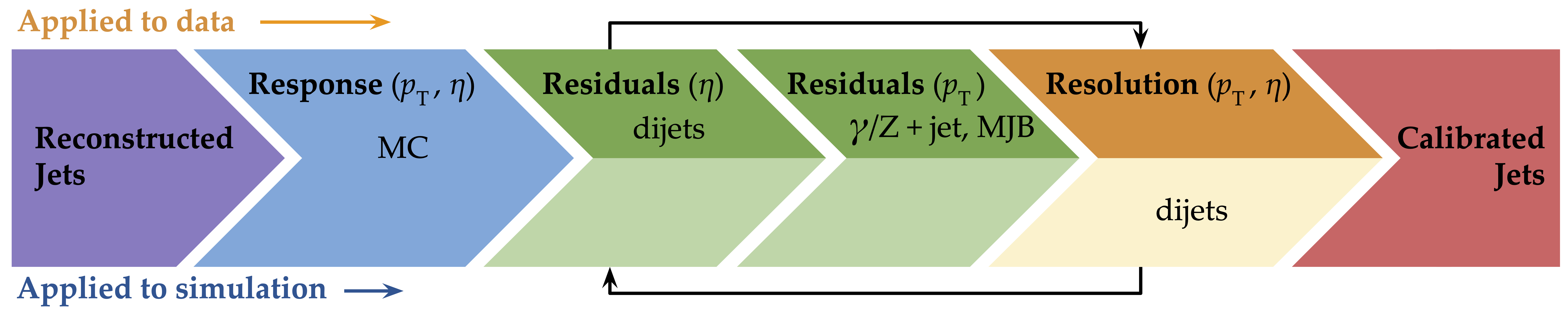
Jets measured from data have typically worse resolution than simulated jets.
Because of this, it is important to ‘smear’ the MC jets with jet energy
resolution (JER) scale factors, so that measured and simulated jets are on
equal footing in analyses. We will demonstrate how to apply the JER scale
factors, since that is applicable for all analyses that use jets.
The resolution is measured in data for different eta bins, and was approximately 10% with a 10% uncertainty for 7 and 8 TeV data.
For precision, it is important to use the correctly measured resolutions,
but a reasonable calculation is to assume a flat 10% uncertainty for simplicity.
Open a notebook
For this part open the notebook called Jet_Energy_Corrections.ipynb and run Exercise 4.
In the notebook, we will use the coffea implementation to apply JER to nanoAOD events.
Notice that the function used to apply corrections will be updated soon to be
compatible with json-pog.
Discussion
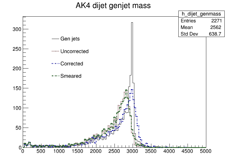
Let’s look at a simple dijet resonance peak shown below.
It corresponds to a dijet resonance peaks analysis. The plot was produced an MC sample of Randall-Sundrum gravitons (RSGs) with m=3 TeV decaying to two quarks. The resulting signature is two high-$p_{\mathrm{T}}$ jets, with a truth-level invariant mass of 3 TeV.
Can you see the effect the correction and the smearing has?
Key Points
The energy of jets in data and simulations is different, for many reasons, and in CMS we calibrate them in a series of steps.
Jets are stochastic objects which its content fluctuates a lot. We measure the jet energy resolution to mitigate this effects.
Jet Substructure
Overview
Teaching: 40 min
Exercises: 20 min
Questions
What is jet substructure?
How to distinguished jets originating from W or top quarks?
Objectives
Learn about high pt ak8jets (FatJet)
Learn about the different substructure variables and taggers
Learn ways to identify boosted W and top quarks
After following the instructions in the setup:
cd <YOUR WORKING DIRECTORY>/notebooks/DAS/
source /cvmfs/sft.cern.ch/lcg/views/LCG_105/x86_64-el9-gcc13-opt/setup.sh
jupyter notebook --no-browser--port=8888 --ip 127.0.0.1
This will open a jupyter notebook tree with various notebooks.
What is a jet?
In the previous episodes we discussed that the jet is a physical object representing the
hadronization of quakrs and gluons. Perhaps we have encounter that a jet can be formed from random
noise or pileup particles in our detectors, not necessarily coming from hard scattered quarks and
gluons, but jets can be so much more:
The internal structure of the jet constituents help us to understand their origin.
Boosted Objects
Heavy particles which are created not at rest but with some momentum are referred as boosted
objects. Let’s analyze the example of a top quark. If the top quarks are boosted, e.g. when coming from a new massive particle, what happens?. Hadronic decay products collimated so then they can be reconstructed in the same final-state object! Hadronic final states now become accessible with a dijet final state (in this case)
Jet mass
QCD jet mass is a perturbative quantity. From the initial (almost) massless partons, pQCD gives rise to a jet mass of order:
[\left< M^2 \right> \simeq C \cdot \frac{\alpha^2}{\pi} p_T^2 R^2]
Jet mass is proportional to R and pT. C is a form factor related to originating parton and clustering algorithm. For non-cone algorithms:
[\left< M^2 \right> \simeq a \times \alpha_S p^2_T R^2]
where $a$ is 0.16 for quarks and 0.37 for gluons. For heavy objects, the LO mass scale is the heavy object mass.
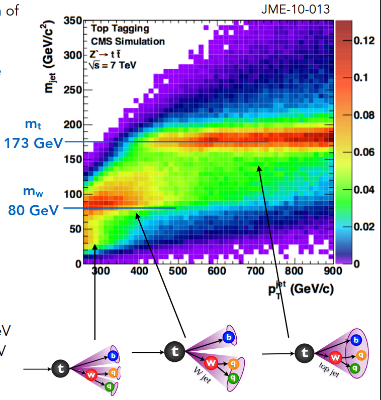
The mass of QCD jets changes as a function of momentum, but the mass of heavy particle jets is relatively stable. For a given mass and pT scale, choose an appropriate jet radius:
[\Delta R \sim \frac{2m}{p_T}]
CMS uses R = 0.8 for heavy object reconstruction. That is merged W/Z at pT ~200 GeV and merged top at pT ~400 GeV.
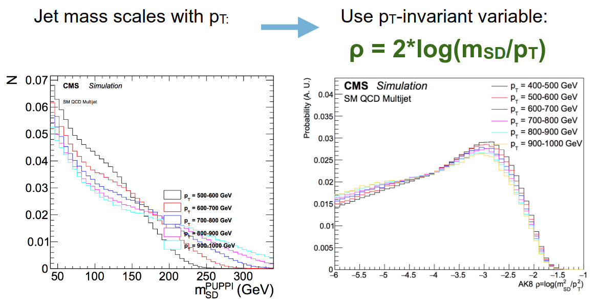
Rho parameter
A useful variable for massive, fat jets is the QCD scaling parameter $\rho$, defined as:
$\rho=\log(m^2/(p_{\mathrm{T}}R)^2)$.
(Sometimes $\rho$ is defined without the log). One useful feature of this variable is that QCD jet mass grows with $p_{\mathrm{T}}$, i.e. the two quantities are strongly correlated, while $\rho$ is much less correlated with $p_{\mathrm{T}}$.
Exercise 4.1
We can use jet mass to distinguish our boosted W and top jets from QCD. Let’s compare the AK8 jet mass of the boosted top quarks from the RS KK sample and the jets from the QCD sample. Let’s also look at the and the softdrop groomed jet mass combined with the PUPPI pileup subtraction algorithm for different samples.
Open a notebook
For this part, open the notebook called Jet_Substructure.ipynb and run Exercise 4.1.
Question 4.1
Do you think the jet mass alone can be used to identify boosted W and top jets?
Question 4.2
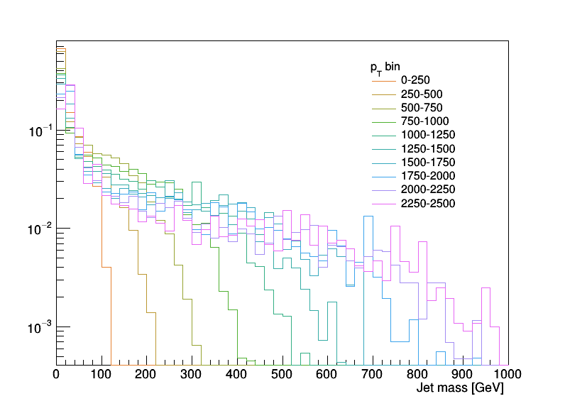
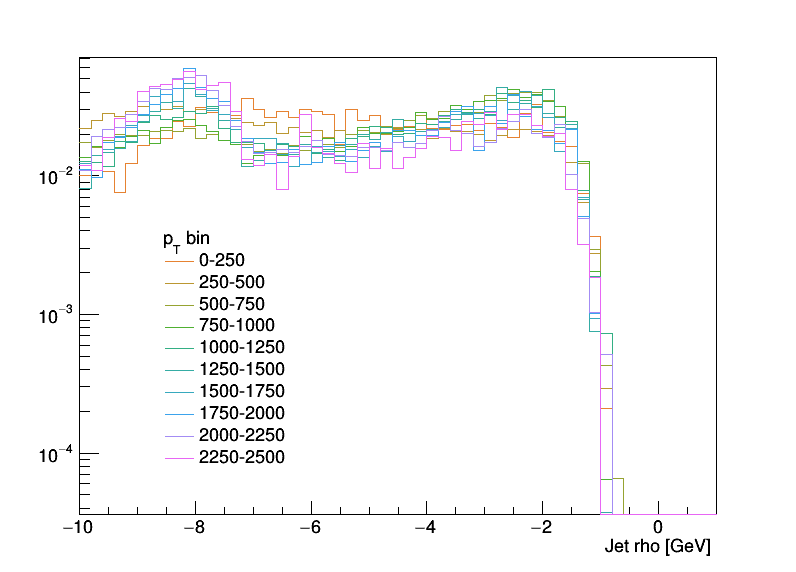
After running Exercise 3, in which cases do you think the $\rho$ variable can be used?
Solution 4.2
The following two plots show what QCD events look like in different $p_{T}$ ranges. It’s clear that the mass depends very strongly on $p_{T}$, while the $\rho$ shape is fairly constant vs. $p_{T}$ (ignoring $\rho<7$ or so, which is the non-perturbative region). Having a stable shape is useful when studying QCD across a wide $p_{T}$ range.
Jet Substructure
Because boosted jets represent the hadronic products of a heavy particle produced with high momentum, some tools have been developed to study the internal structure of these jets. This topic is usually called Jet Substructure.
Jet substructure algorithms can be divided into three main tools:
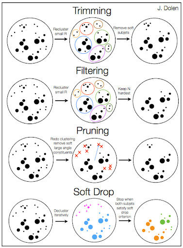
grooming algorithms attempt to reduce the impact of soft contributions to clustering sequence by adding some other criteria. Examples of these algorimths are softdrop, trimming, pruning.
subtructure variables are observables that try to quantify how many cores or prongs can be identify within the structure of the boosted jet. Examples of these variables are n-subjetiness or energy correlation functions.
taggers are more sofisticated algorithms that attempt to identify the origin of the boosted jet. Currently taggers are based on sofisticated machine-learning techniques which try to use as much information as possible in order to efficiency identify boosted W/Z/Higgs/top jets. Examples of these taggers in CMS are deepAK8/ParticleNet or deepDoubleB.
For further reading, several measurements have been performed about jet substructure:
There has been many different approaches to jet grooming during the years. The standard idea is to remove soft and wide-angle radiation from within the jet, then recluster with smaller R, remove subjets and then remove constituents during clustering.
The next cartoon provides a good summary of all these algorithms:
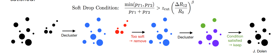
The softdrop algorithm is the one choosen at CMS by default. Softdrop recursively decluster jet. Remove the softer component unless the soft drop condition is
satisfied.
Soft wide angle radiation fails the condition:
As $z_{cut}$ increases, then more aggressive grooming
As $\beta$ decreases, then more aggressive grooming
Example (zcut = 0.1) :
If $\beta =0$, remove softer subjet if pT fraction < 0.1 (~equivalent to MMDT)
If $\beta > 0$, remove softer subjet if pT fraction < x, where x increases with ΔR and has maximum value 0.1
If $\beta \lim \infty$ no grooming
If $\beta <0$ soft drop becomes a tagger instead of a groomer (finds jets with hard, large angle subjets)
Jet grooming algorithms dramatically improves the separation of QCD and top quark jets. Merged top quarks can be identified with a window around the top quark mass.
Exercise 4.2
In this part of the tutorial, we will compare different subtructure algorithms as well as some usually subtructure variables.
Open a notebook
For this part, open the notebook called Jet_Substructure.ipynb and run Exercise 4.2.
Question 4.3
Look at the following histogram, which compares ungroomed, pruned, soft drop (SD), PUPPI, and
SD+PUPPI jets.
Note that the histogram has two peaks. What do these correspond to? How do the algorithms affect the relative size of the two populations?
Substructure variables
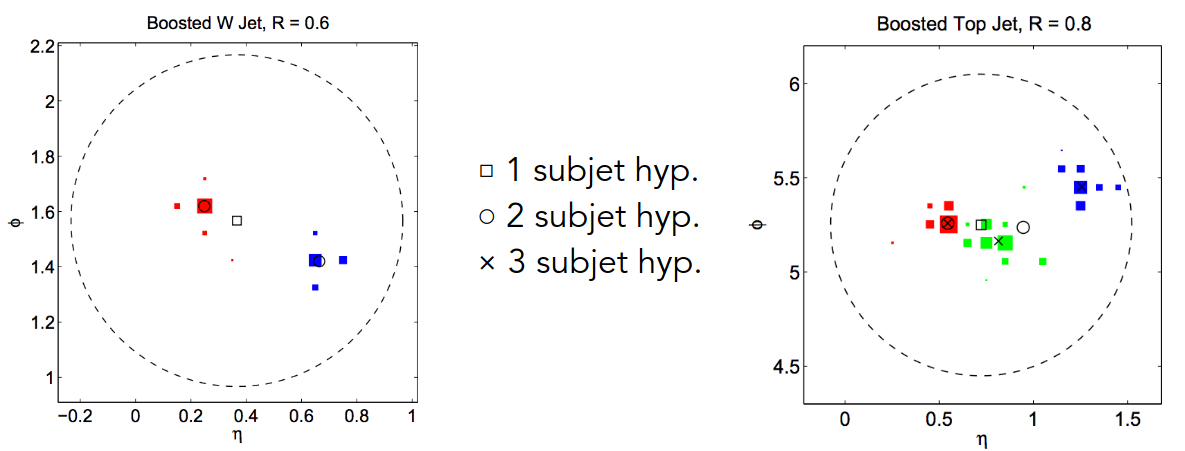
Knowing how many final state objects to expect from these decays we can look inside the jet for the expected substructure:
Top decays → 3 subjets
W/Z/H decays → 2 subjets
*
A quantity called N-subjettiness is a measure of how consistent a jet is with a hypothesized number of subjets. N-subjetiness is defined as:
The variable $\tau_N$ gives a sense of how many N prongs or cores can be find inside the jet. It is known that the n-subjetiness variables itself ($\tau_{N}$) do not provide good discrimination power, but its ratios do. Then, a $\tau_{MN} = \dfrac{\tau_M}{\tau_N}$ basically tests if the jet is more M-prong compared to N-prong. For instance, we expect 2 prongs for boosted jets originated from hadronic Ws, while we expect 1 prongs for high-pt jets from QCD multijet processes. The most common nsubjetiness ratio are $\tau_{21}$ and $\tau_{32}$.
Another subtructure variable commonly used is the energy correlation function $N2$. Similarly than $\tau_{21}$, $N2$ tests if the boosted jet is compatible with a 2-prong jet hypothesis.
Exercise 4.3
Open a notebook
For this part, open the notebook called Jet_Substructure.ipynb and run Exercise 4.3.
Question 4.4
Look at the histogram comparing $\tau_{21}$. What can you say about the histogram? Is $\tau_{21}$ telling you something about the nature of the boosted jets selected?
Question 4.5
Look at the histogram comparing $\tau_{32}$. What can you say about the histogram? Is $\tau_{32}$ telling you something about the nature of the boosted jets selected?
Question 4.6
Look at the histograms comparing $N2$ and $N3. What can you say about the histogram? Are these variables telling you something about the nature of the boosted jets selected?
Taggers
In this part of the tutorial, we will look at how different substructure algorithms can be used to identify jets originating from boosted W’s and tops. Specifically, we’ll see how these identification tools are used to separate these boosted jets from those originating from Standard Model QCD, a dominant process at the LHC.
W tagging
top tagging
Tagging with machine learning
W/Top tagging was one of the first places where ML was adopted in CMS. We have study several of these algorithms (JME-18-002), being “deepAK8/ParticleNet” the most used within CMS.
Exercise 4.4
Open a notebook
For this part, open the notebook called Jet_Substructure.ipynb and run Exercise 4.4.
Question 4.7
Why can we use a ttbar sample to talk about W-tagging?
What cuts would you place on these variables to distinguish W bosons from QCD?
So far, which variable looks more promising?
Question 4.8
What cut would you apply to select boosted top quarks?
For both the W and top selections, what other variable(s) could we cut on in addition?
Go Further
You can learn more about jet grooming from the jet substructure exercise and PUPPI from the pileup mitigation exercise.
We briefly mentioned that you can combine variables for even better discrimination. In CMS, we do this to build our jet taggers. For the simple taggers, we often combine cuts on jet substructure variables and jet mass. The more sophisticated taggers, which are used more and more widely within CMS, use deep neural networks. To learn about building a machine learning tagger, check out the machine learning short exercise. (FIXME)
What about boosted Higgs?
CMS has also a rich program for booted Higgs to bb/cc taggers, however they are usually studied by
the btagging group (BTV). Look at their documentation for more information.
Key Points
Jet substructure is the field study the internakl structure of high pt jets, usually clustered with a bigger jet radius (AK8).
Grooming algorithms like softdrop, and substructure variables like the nsubjettiness ratio help us to identify the origin of these jets.
Over the years more state-of-the-art taggers involving ML have been implemented in CMS. Those help us indentify more effectively boosted jets.
Missing Transverse Energy 101
Overview
Teaching: 20 min
Exercises: 10 min
Questions
What is MET? How is MET reconstructed?
What are the types of MET at CMS?
Examples of analyses with MET at CMS
Objectives
Learn about MET, the definition, types and reconstruction algorithms.
Learn about extracting MET in MiniAOD files.
After following the instructions in the jets exercise setup, make sure you have the CMS environment and create the symbolic link to MET analyzer:
cd$CMSSW_BASE/src/Analysis
cmsenv
Event Reconstruction
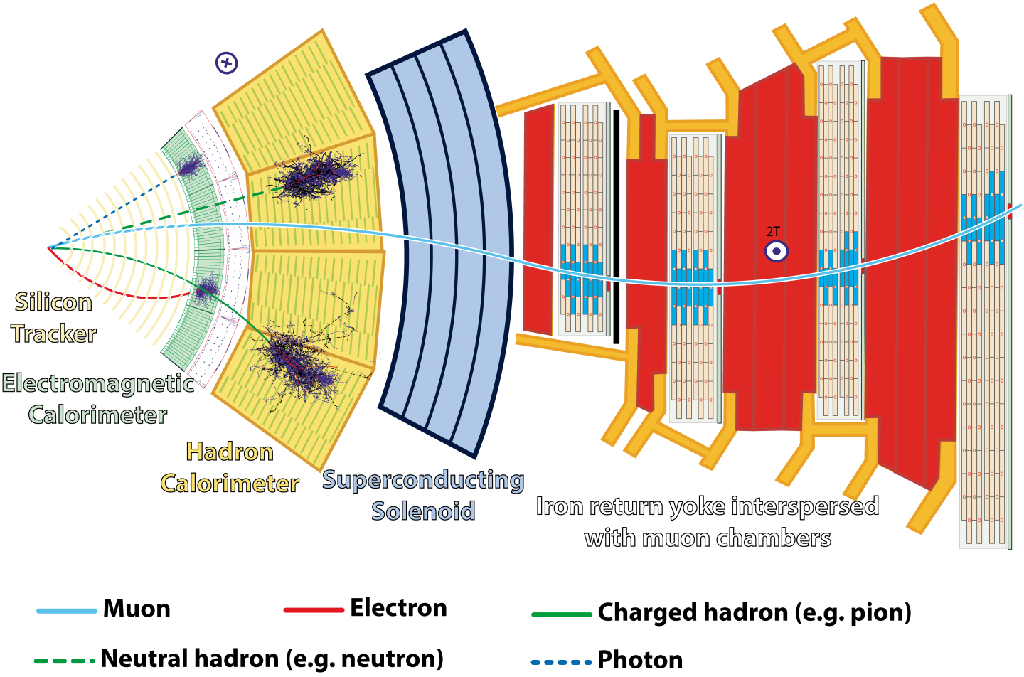
Event reconstruction in CMS is achieved using the Particle Flow (PF) algorithm, which integrates information from all CMS subdetectors to reconstruct individual particles.
The algorithm produces a list of PF candidates classified as electrons, photons, muons, neutral hadrons, or charged hadrons.
These PF candidates are then used to reconstruct high-level physics objects, including jets and missing transverse momentum (MET).
Schematic of the CMS particle flow reconstruction algorithm.
Missing Transverse Energy
MET quantifies the imbalance in the transverse momentum of all visible particles in the final state of collisions—those interacting via electromagnetic or strong forces.
Due to momentum conservation in the transverse plane (the plane perpendicular to the beam), MET reflects the transverse momentum carried by undetected weakly interacting particles, such as neutrinos or potential dark matter candidates.
Although these invisible particles leave no direct signature in the CMS detector, their presence is inferred from the observed net momentum imbalance in the event.
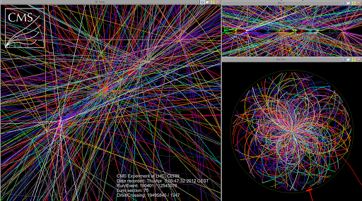
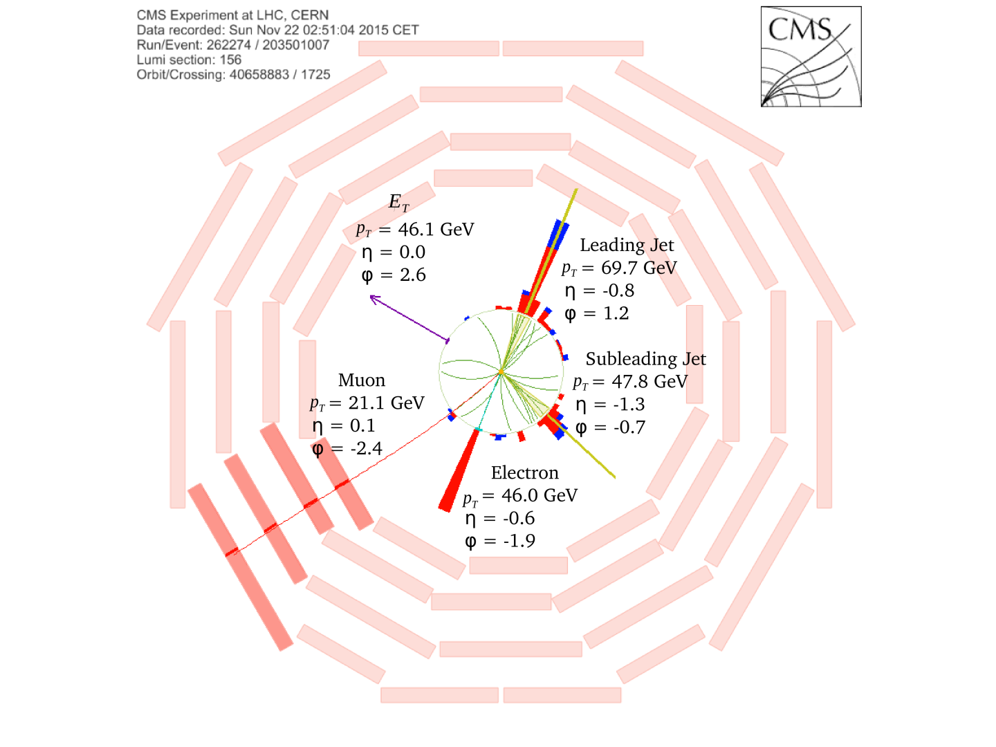
An example of event with MET is shown in the figure below where two top quarks are produced. Each top quark decays into a b-jet and a W boson. The leptonic decay of a W boson leads to a lepton and its corresponding neutrino. So, the final state contains two jets, two leptons and missing transverse energy from two neutrinos.
Event display of a ttbar event recorded by CMS shows the dileptonic decay channel with two jets, one electron, one muon, and missing transverse energy from two neutneutrinosrinoes.
MET is a vital variable in many CMS analyses, playing a key role in both Standard Model measurements and Beyond Standard Model searches.
In the Standard Model, MET is used to study processes involving neutrinos in the final state, such as the W boson mass measurement.
In searches for new physics, MET helps identify potential signatures where weakly interacting particles escape detection, such as dark matter, resulting in an imbalance in transverse momentum.
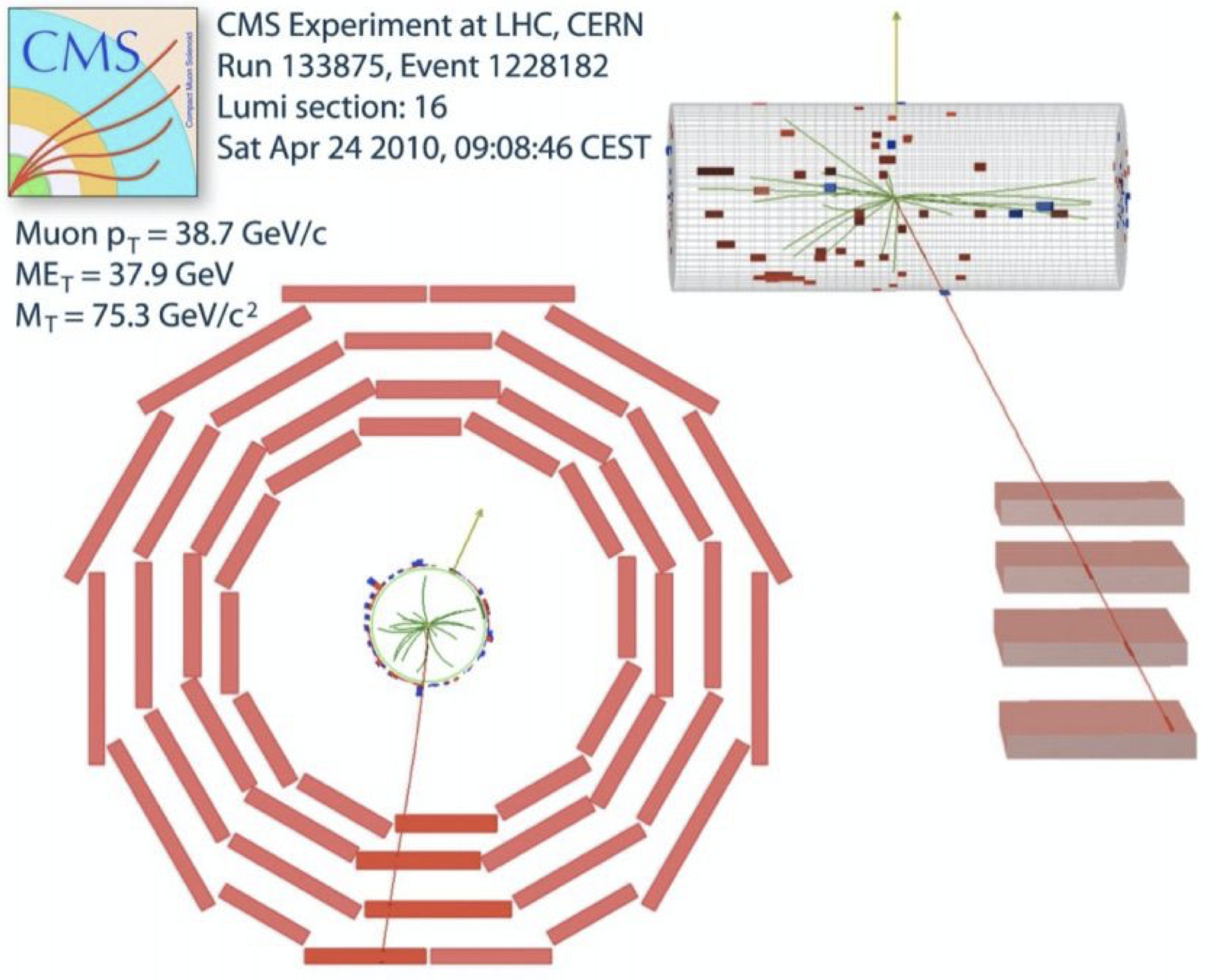
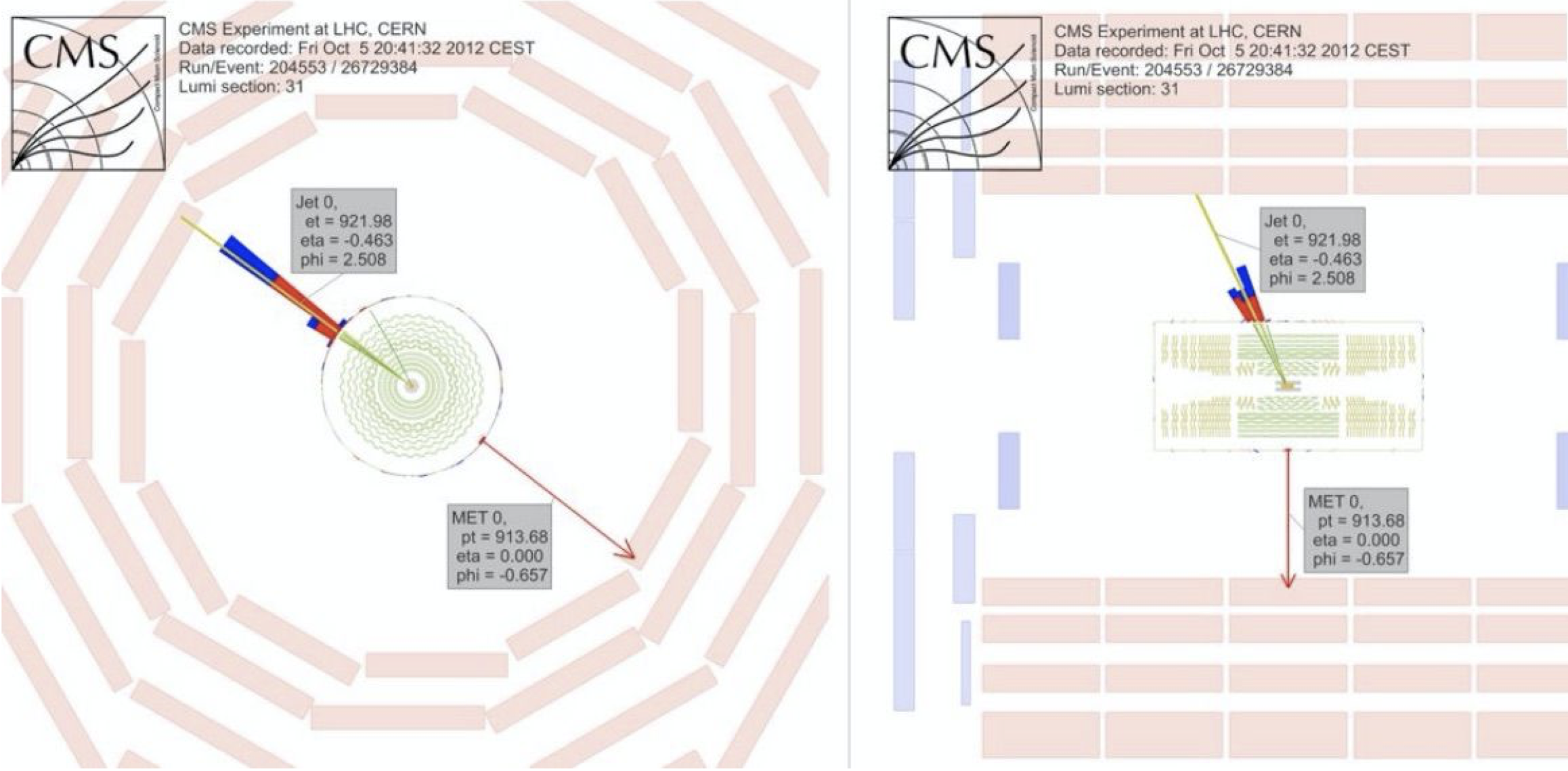
The images below illustrate two such cases: on the left, a candidate W boson event with $W \rightarrow \mu \nu$, used in the W mass measurement, and on the right, a candidate event for dark matter production, featuring a hard jet recoiling against large missing energy.
W boson candidate event with a muon and neutrino.Dark matter search event with a hard jet recoiling against large MET.
Event displays of analyses involving MET.
Raw PF MET
The most widely used MET reconstruction algorithm in CMS is the PF MET.
PF MET is reconstructed as the negative vector sum of the pT of all PF candidates in the event, which is summarized in the following equation:
Multiple simultaneous proton-proton collisions occurring in the same bunch crossing, referred to as pileup, adversely affect MET resolution, leading to poorer performance at higher pileup levels. To mitigate these effects and improve MET performance with respect to pileup, CMS employs an alternative reconstruction algorithm known as PUPPI MET.
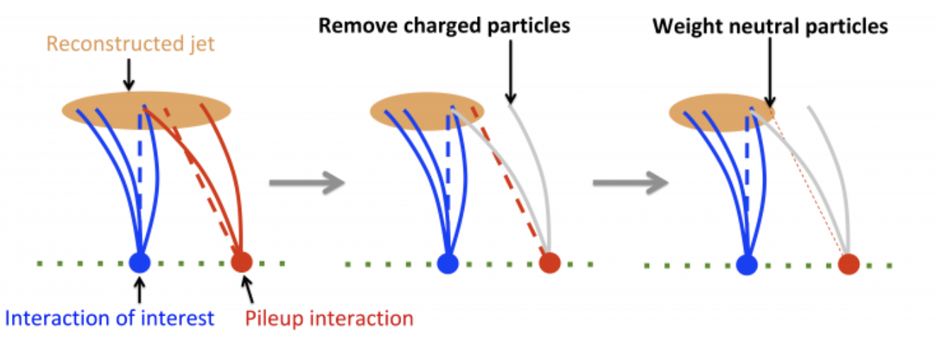
The PUPPI (Pileup Per Particle Identification) algorithm applies inherently local corrections by leveraging specific properties of particles. Particles originating from the hard scatter process are typically geometrically close to other particles from the same interaction and generally exhibit higher pT. In contrast, pileup particles lack shower structures, have lower pT on average, and are uncorrelated with particles from the leading vertex.
Using this information, the PUPPI algorithm removes charged particles associated with pileup vertices and assigns weights (ranging between 0 and 1) to neutral particles based on their likelihood of originating from pileup, thus enhancing MET reconstruction in high-pileup environments. The PUPPI MET is calculated using particle weights and can be summarized in the following equation:
The figure below presents the MET distribution for both PF MET and PUPPI MET in events with leptonically decaying W bosons, demonstrating the improved performance achieved with PUPPI MET.
Remember
PUPPI MET is the default MET algorithm in Run~3.
Exercise 1
The goal of this part is to get familiar:
with the event content of the miniAOD data tier,
the MET collections stored by default in miniAOD,
how to use tools to easily browse through the miniAOD file.
To view the event content of a miniAOD file one can use the edmDumpEventContent command and since we are interested in the MET collections only we use grep to avoid long printouts.
edmDumpEventContent root://eosuser.cern.ch//eos/user/c/cmsdas/2025/MET/DYJetsToLL_M50_amcatnloFXFX.root | grep MET
Question 1
What MET collections do you see inside a MiniAOD file?
Each entry (line) corresponds to a separate MET collection.
The first column, pat::MET, shows the class of the MET object, where one finds the properties of the MET object.
The second column shows the MET collection, and finally PAT is the namespace (in MiniAOD it is PAT).
In this exercise we will focus on the slimmedMETs and slimmedMETsPuppi collections.
Key Points
Weakly interacting neutral particles produced in proton-proton (pp) collisions at the LHC traverse the CMS detector unobserved.
Their presence is inferred from the measurable momentum imbalance in the plane perpendicular to the beam direction when produced alongside electromagnetically charged or neutral particles. This measurable transverse momentum imbalance is referred to as missing transverse momentum (MET).
Precise determination of MET is critical for Standard Model measurements involving final states with neutrinos and searches for physics beyond the SM targeting new weakly interacting particles.
MET reconstruction is sensitive to experimental resolutions and mis-measurements of reconstructed particles, detector artifacts, and the effects of additional pp interactions within the same or nearby bunch crossings (pileup).
MET Calibrations
Overview
Teaching: 20 min
Exercises: 10 min
Questions
Why do we need to calibrate MET? How is the performance measured?
What are the different ways of calibrating MET at CMS?
What is MET phi modulation? How to correct for it?
How is the uncertainty on MET estimated?
Objectives
Learn about the MET calibration procedure and techniques used at CMS.
Learn about measuring MET performance.
Understand MET phi modulation and how to account for it.
Learn about MET uncertainty sources and to get the MET uncertainty in MiniAOD analyses.
After following the instructions in the setup, make sure you have the CMS environment:
The MET objects described earlier (PF-MET and PUPPI-MET) are referred to as raw MET, and they are systematically different from the true MET, which corresponds to the transverse momentum carried by invisible particles.
This difference arises from factors such as the non-compensating nature of the calorimeters, calorimeter thresholds, and detector misalignment, among others.
To improve the MET estimate and make it closer to the true MET, corrections can be applied.
Type-1 Correction
The Type-I correction is the most commonly used MET correction in CMS.
It propagates the jet energy corrections (JEC) to MET. Specifically, the Type-I correction replaces the vector sum of the transverse momenta of particles clustered as jets with the vector sum of the transverse momenta of the jets, which have been corrected with JEC.
Particles can be classified into two disjoint sets: those that are clustered as jets and those that remain unclustered.
The superscript “uncorr” indicates that the jet energy correction (JEC) has not yet been applied to these jets.
The Type-I correction replaces the raw jet pT with the corrected jet pT. The Type-I correction can be expressed as the difference between two vector sums:
We will revisit this in MET performance, but this figure shows a comparison between the MET scale for raw and Type-1 corrected MET.
Type-1 Smear MET (For MC only)
In MC simulations, jets are smeared to achieve better agreement with data. This smearing of MC jets can additionally be propagated to MET, resulting in Type-1 smear MET.
Remember
PF MET is the recommended MET algorithm in Run 2, and PUPPI MET is recommended for Run 3 analyses.
Type-I corrected MET is the default MET calibration required in all analyses.
XY corrections
The XY correction reduces the MET $\phi$ modulation. This correction also helps mitigate pile-up effects.
The distribution of true MET is independent of $\phi$ due to the rotational symmetry of collisions around the beam axis.
However, we observe that the reconstructed MET does depend on $\phi$.
The MET $\phi$ distribution follows roughly a sinusoidal curve with a period of $2\pi$.
The possible causes of this modulation include:
Anisotropic detector responses
Inactive calorimeter cells
Detector misalignment
Displacement of the beam spot
The amplitude of the modulation increases roughly linearly with the number of pile-up interactions.
For example, following plot shows the MET $\phi$ distribution without the XY correction in events with an electron and a muon where $t\bar{t}$+jets background dominates:
After applying the correction the data/MC agreement improves:
MET Uncertainty
For analyses sensitive to missing transverse energy — those involving large MET contributions from neutrinos or other signatures — it is necessary to break MET into its individual components.
Since MET is calculated as the vector sum of contributions from jets, electrons, muons, taus, photons, and “unclustered energy” (energy not associated with reconstructed objects), the resolution and scale of each component must be propagated to MET.
These uncertainties are then treated as separate nuisance parameters each arising from a different physics object.
The physics objects that contribute the most are:
Jets: Jet energy scale (JES) and jet energy resolution (JER) uncertainties directly impact MET, as jets typically contribute significantly to the total energy.
Unclustered Energy: Unclustered energy includes contributions from particles not grouped into jets, leptons, or photons. The uncertainty arises from the resolution of individual particle types, such as charged hadrons, neutral hadrons, photons, and hadronic forward (HF) particles.
Leptons: This includes tau leptons, electrons, muons, and photons. Scale uncertainties for these objects need to be propagated to MET, as even small variations can affect its calculation.
The scale and resolution of each component must be systematically varied within their respective uncertainties. These variations are then propagated to the MET calculation to calculate their impact on the analysis.
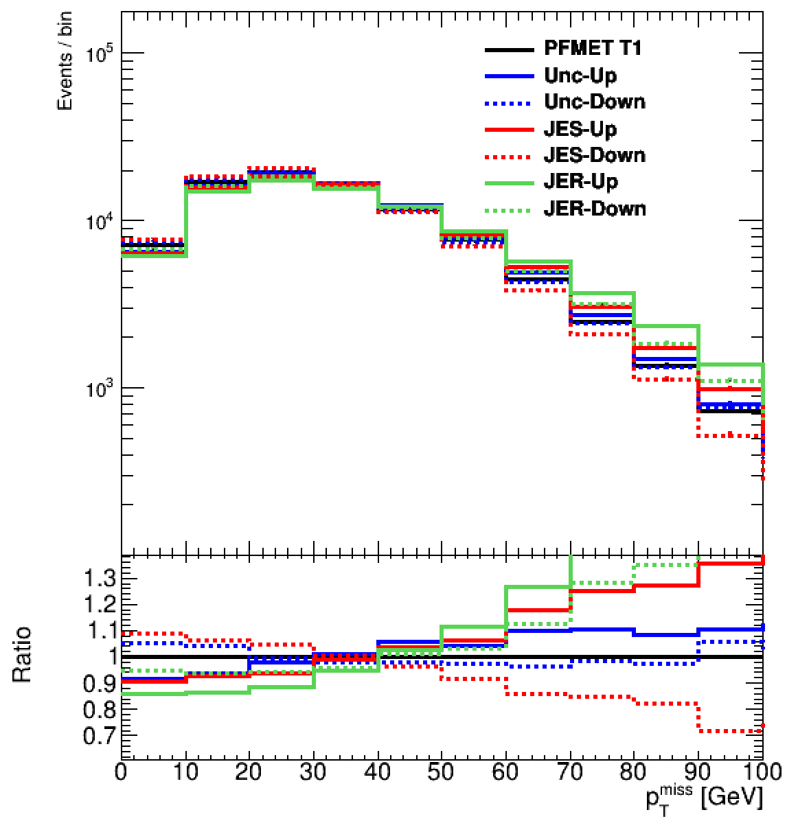
Following figure shows the distribution of the Type 1 corrected MET reconstructed by the PF algorithm in MC and in data along with the uncertainties in the ratio plot.
Exercise 2.1
In this section, we will focus on accessing the MET object(s) in miniAOD, including:
Different MET calibrations
MET uncertainties
Firstly, we will access different MET flavors: the raw PFMET, the Type-1 PFMET (the default MET flavor in CMS), and the Type-1 smeared PFMET.
In Type-1 MET, corrections from the jet energy scale are propagated to MET, whereas in Type-1 smeared MET, corrections from both the jet energy scale and the jet energy resolution are applied.
MET relies on accurate momentum/energy measurements of reconstructed physics objects, including muons, electrons, photons, hadronically decaying taus, jets, and unclustered energy (UE). The latter refers to contributions from PF candidates not associated with any of the previously mentioned physics objects.
Since uncertainties in MET measurements strongly depend on the event topology, uncertainties in the momenta of all reconstructed objects are propagated to MET. This is done by varying the momentum estimate of each object within its uncertainty and recomputing MET.
In this exercise, we will consider three sources of uncertainty:
Jet energy scale
Jet energy resolution
Unclustered energy
We will use the same file as in the previous exercise Exercise 1.1.
Execute the following commands inside the CMSSW environment created during setup:
Print the transverse momentum ($p_T$) and azimuthal angle ($\phi$) of the MET object for each event
Print the values of various sources of systematic uncertainties
Additionally, the script demonstrates how to access MET with different levels of corrections applied. By default, Type-1 MET is selected.
The analyzer being run using is command is JMEDAS/plugins/CMSDAS_MET_AnalysisExercise2.cc. The printout looks like the following:
Begin processing the 1st record. Run 1, Event 138728702, LumiSection 513811 on stream 0 at 05-Jan-2025 14:40:03.942 CST
 MET :
  pt [GeV] = 4.42979
  phi [rad] = 2.92774
 MET uncertainties :
  JES up/down [GeV] = 2.22909/6.63454
  JER up/down [GeV] = 4.34603/4.51426
  Unc up/down [GeV] = 9.2058/6.06604
 MET corrections :
  Raw PFMET pt [GeV] = 10.7137
  PFMET-type1 pt [GeV] = 4.42979
  Smeared PFMET-type1 pt [GeV] = 4.40847
  .......
  .......
Question 2.1
Compare the distributions of the above quantities and get a feeling about their effect. Wheer are these distrucutions being stored?
Solution 2.1
The various MET histograms (raw, Type-1, JES Up, JER down etc.) are being stored at ./outputs/cmsdas_met_exercise2.root
Exercise 2.2
Now we make the following modifications to the configuration script JMEDAS/test/run_CMSDAS_MET_Exercise2_cfg.py:
Prevent printouts by setting doprints to False.
Reduce the frequency of the report from “every” event to “every 10000” events by modifying process.MessageLogger.cerr.FwkReport.reportEvery.
Run over all events in the file by updating process.maxEvents from 10 to -1.
After these modifications, please re-run the configuration with the following command:
cmsRun test/run_CMSDAS_MET_Exercise2_cfg.py
Once the process completes (it will take a few seconds), it will produce a ROOT file. We will then compare the 1D distribution of different MET flavors in a Z+jets sample (which has no genuine MET).
To generate the plot, run the following commands:
What do you observe looking at the different MET calibration algorithms?
Solution 2.2
Exercise 2.3
Next, we will focus on Type-1 PF MET and study the impact of various uncertainties, including Unclustered, JES, and JER.
To generate the corresponding plot, use the following command:
What do you observe looking at the different sources of MET uncertainty?
Solution 2.3
Key Points
Inaccurate MET estimation can result from sources such as non-linearity in the calorimeter’s response to hadrons, minimum energy thresholds in the calorimeters, and pT thresholds or inefficiencies in track reconstruction. These issues are mitigated through calibration procedures discussed in this exercise.
Type-1 MET is the default MET calibration recommended by CMS.
Type-1 smear MET enhances data-MC agreement, and JME POG advises analysts to assess its impact in their studies.
MET is influenced by uncertainties from all contributing objects, including jets, leptons, photons, and unclustered energy. Systematic variations in the scale and resolution of each component must be propagated to the MET calculation to evaluate their impact on the analysis.
MET performance
Overview
Teaching: 20 min
Exercises: 10 min
Questions
How do we measure the MET performance (i.e. MET scale and MET resolution) ?
Objectives
Learn about MET performance.
Measure the resolution and scale of MET for different MET algorithms and calibrations.
After following the instructions in the setup, make sure you have the CMS environment:
cd$CMSSW_BASE/src/Analysis
cmsenv
MET performance
A well-measured Z boson or photon provides a unique event axis and a precise momentum scale for evaluating MET performance.
To achieve this, the response and resolution of MET are studied in samples where a Z boson decays to a pair of electrons or muons, or in events with an isolated photon.
Such events should have little to no genuine MET.
The MET performance is then assessed by comparing the momentum of the vector boson to that of the hadronic recoil system.
The hadronic recoil system is defined as the vector sum of the transverse momenta of all PF candidates, excluding the vector boson (or its decay products in the case of Z boson decay).
Momentum conservation in the transverse plane imposes
where \(\vec{q}_{T}\) is the transverse momentum of the Z boson, and \(\vec{u}_{T}\) is the hadronic recoil.
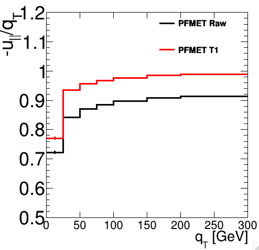
Define two components of the hadronic recoil to study the MET response and resolution:
hadronic recoil parallel (\(u_{\parallel}\)) to the boson axis: sensitive to the scale of boson/jets
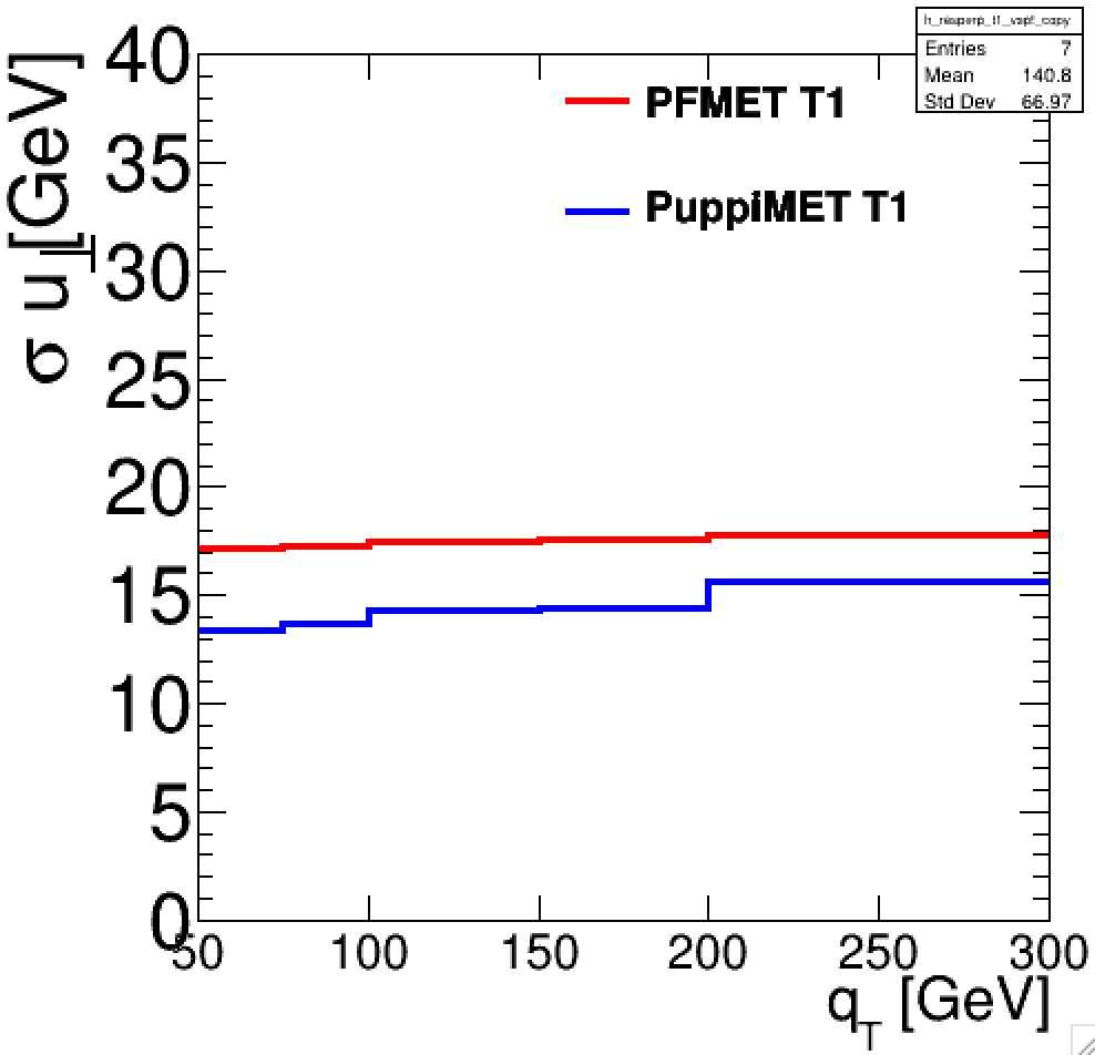
perpendicular (\(u_{\perp}\)) to the boson axis: sensitive to isotropic effects like pileup
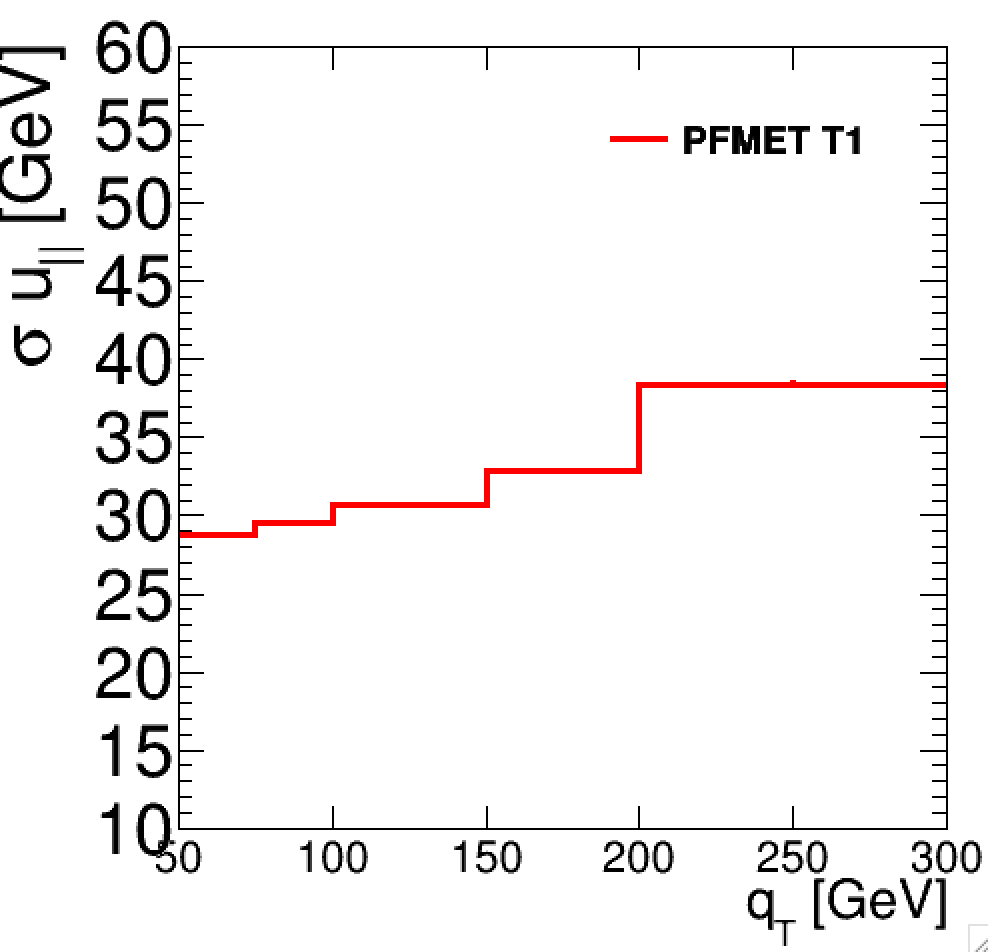
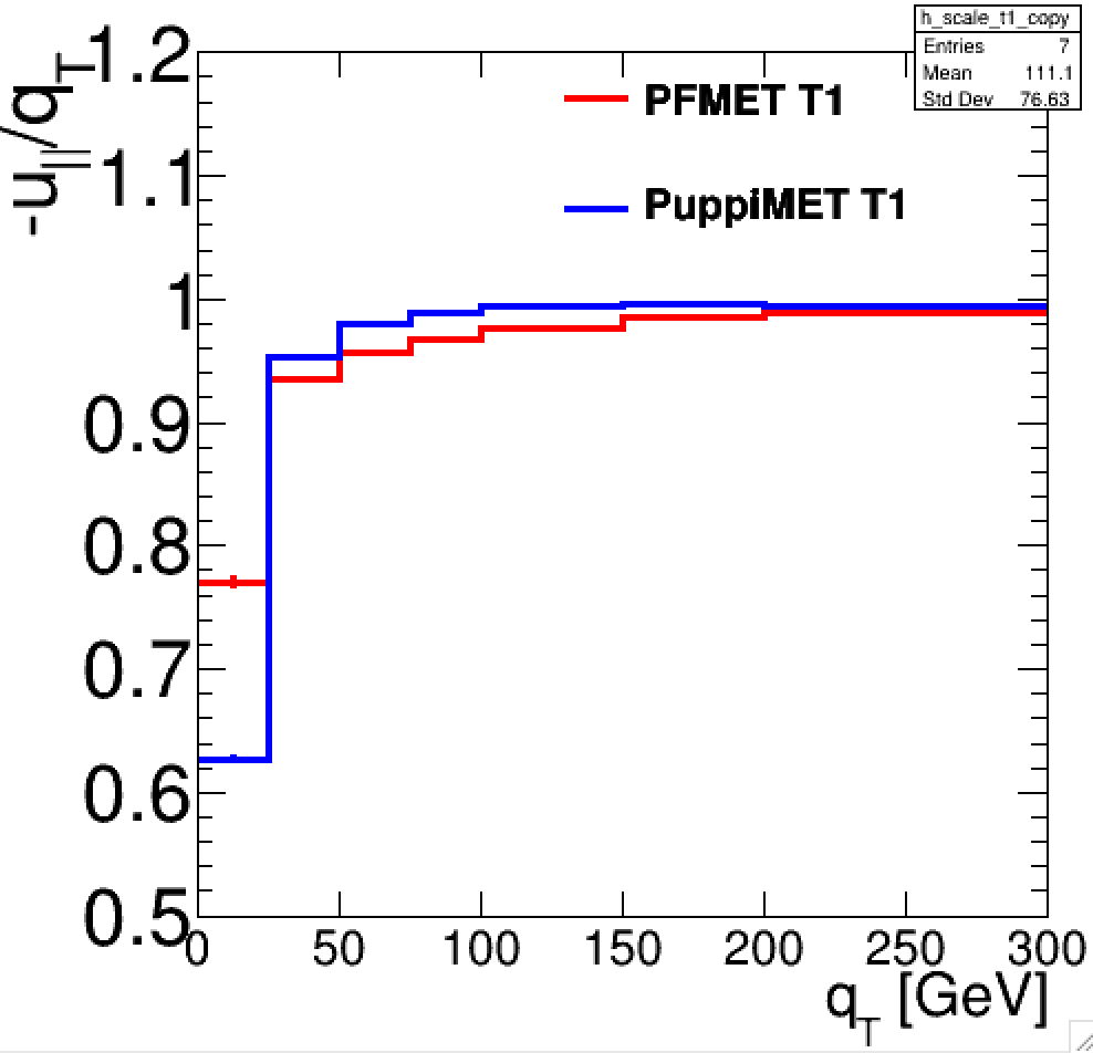
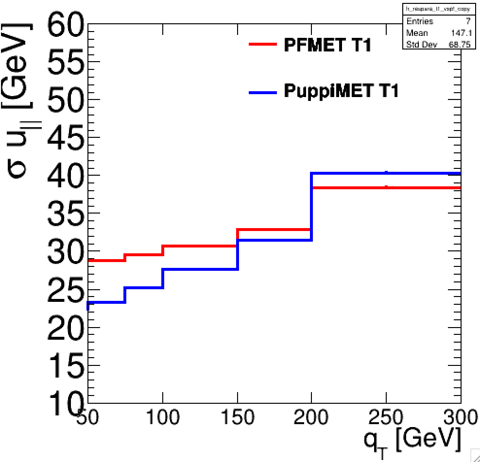
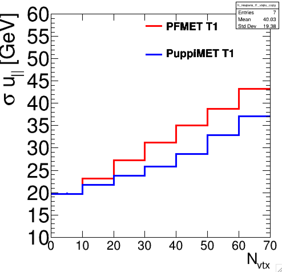
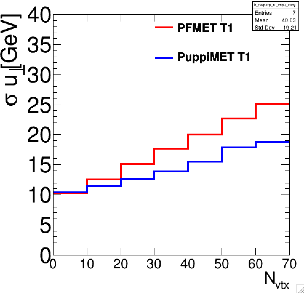
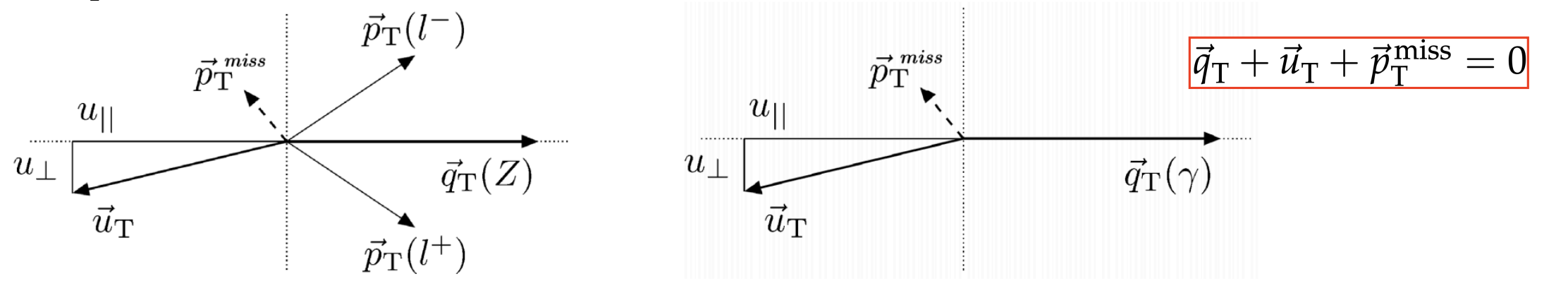
Specifically, the mean of the distribution of the magnitude of \(q_{T} + u_{\parallel}\), is used to estimate the MET response, whereas the RMS of \(q_{T} + u_{\parallel}\) and \(u_{\perp}\) distributions are used to estimate the MET resolution in the axis parallel and perpendicular to the Z boson, respectively.
An example of the \(q_{T} + u_{\parallel}\) and $u_{\perp}$ distributions is shown in the following plots.
Use the distribution of the parallel and perpendicular components of the hadronic recoil to measure the MET scale and resolution
Get the mean of the parallel component to estimate MET scale.
The RMS of the distributions gives the MET resolution in each direction.
Exercise 3.1: MET Scale
In this exercise, we will measure the scale of the “uncorrected” (raw) PF MET as a function of the transverse momentum of the Z boson (pT(Z)).
For a fully calibrated MET object, what behavior would you expect to see in the distribution?
Solution 3.1 (a)
For a fully calibrated MET object, the scale is expected to be approximately 1, indicating an accurate representation of the true missing transverse energy with minimal systematic bias.
Next, measure the MET scale using the Type-1 calibrated MET. Run the following commands:
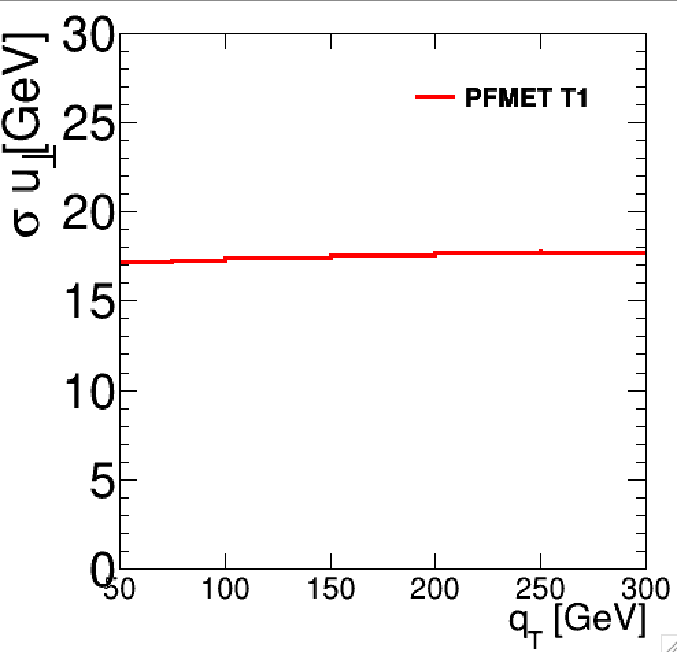
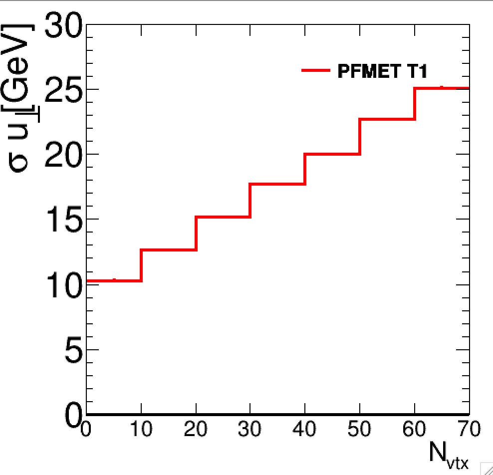
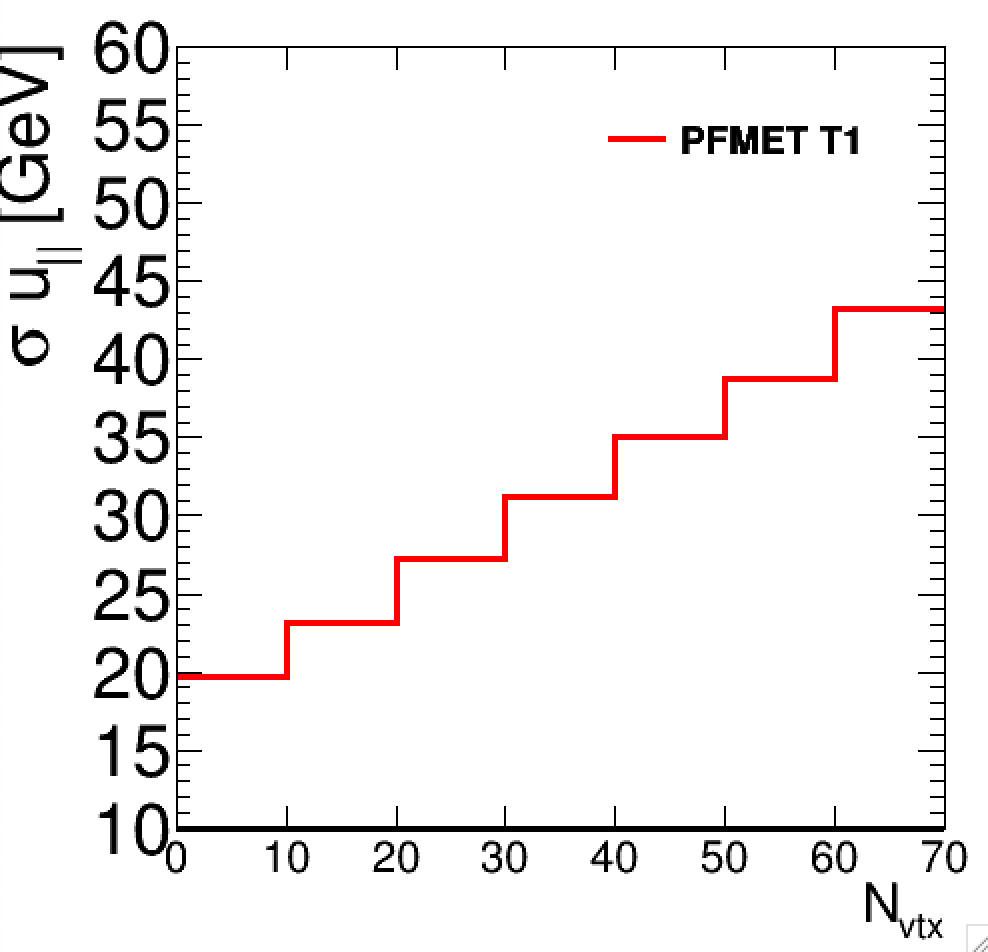
This command will generate distributions showing the resolution of the parallel ($u_{\parallel}$) and perpendicular ($u_{\perp}$) components of MET with respect to pT(Z) and pileup.
Question 3.2
How does the MET resolution depend on pileup?
Solution 3.2
The MET resolution degrades significantly as pileup increases, with an average deterioration of approximately 4 GeV per additional pileup vertex.
For more detailed insights, refer to the CMS MET paper based on 13 TeV data: CMS-JME-17-001.
Exercise 3.3
Equipped with the ability to evaluate MET performance through scale and resolution, we now aim to compare Type-1 PF MET with Type-1 PUPPI MET. Starting from Run 3, Type-1 PUPPI MET is the default MET algorithm in CMS. In this example, we will examine the performance of PF MET and PUPPI MET by comparing their scale and resolution.
To generate the corresponding plots, use the following command:
Compare the correlation between Type1 PFMET and Puppi MET. What do you observe?
Solution 3.3 (a)
Question 3.3 (b)
Compare the scale and resolution between Type1 PFMET and Puppi MET, especially the resolution as a function of \(N_{vtx}\). What do you observe?
Solution 3.3 (b)
Significantly improved MET resolution as a function of \(N_{vtx}\) compared to PFMET.
PUPPI-MET has 2x smaller degradation in resolution compared to PFMET.
Key Points
The performance of MET is studied in events with a well-measured Z boson (decaying to electrons or muons) or an isolated photon, which should have little to no genuine MET.
Transverse momentum conservation is used to study MET response and resolution along z-axis.
Handling Anomalous MET Events
Overview
Teaching: 20 min
Exercises: 10 min
Questions
What is anomalous MET?
How to identify these events?
Objectives
Learn about anomalous MET
Learn about the Noisy event filters and their implementation.
After following the instructions in the setup, make sure you have the CMS environment:
cd$CMSSW_BASE/src/Analysis
cmsenv
What is anomalous MET?
Anomalous MET refers to events where the measured MET deviates from what is expected due to various factors, such as reconstruction failures, detector malfunctions, or background noise.
These anomalous MET events can arise from:
Detector Issues: Malfunctions or mismeasurements in detectors, such as the electromagnetic calorimeter (ECAL) or hadronic calorimeter (HCAL), leading to spurious energy deposits.
Reconstruction Failures: Errors in reconstructing particle tracks or energy, including issues with jets, leptons, or unclustered energy, that result in inaccurate MET calculations.
Non-collision Origins: Spurious signals from sources unrelated to the particle collision, such as beam-halo particles, cosmic rays, or other environmental factors.
Dead or Malfunctioning Detector Cells: Areas of the detector that fail to register energy deposits correctly, leading to underestimation of the MET.
In such events, the MET value may be much higher than expected and does not reflect true missing energy from invisible particles (like neutrinos or dark matter candidates).
An example of identifying the source of anomalous MET.
Noisy event filters
To identify false MET, several algorithms have been developed that analyze factors such as timing, pulse shape, and signal topology.
When fake MET is detected, the corresponding events are typically discarded.
These cleaning algorithms, or filters, run in separate processing paths, and the outcome (success or failure) is recorded as a filter decision bit.
Analyzers can use this decision bit to filter out noisy events. These filters are specifically designed to reject events with unusually large MET values caused by spurious signals.
MET $p_T$ and leading jet $\phi$ distributions, with and without the application of event filters.
Excercise 4
Noisy event filters (previously called MET Filters) are stored as trigger results, specifically in edm::TriggerResults of the RECO or PAT process. Each MET filter runs in a separate path, and the success or failure of the path is recorded as a filter decision bit. For more information, please refer to the provided link.
In this exercise, we will show how to access the MET Filters in miniAOD. Please run the following commands:
This example accesses the decision bits for the following MET Filters: Beam Halo, HBHE, HBHE (Iso), Ecal Trigger Primitives, EE SuperCluster, Bad Charged Hadron, and Bad PF Muon. A “true” decision means the event was not rejected by the filter. The analyzer used in this example is JMEDAS/plugins/CMSDAS_MET_AnalysisExercise5.cc. The printed result will look like this:
Begin processing the 1st record. Run 317626, Event 178458435, LumiSection 134 on stream 0 at 28-Jun-2020 10:39:20.656 CDT
MET Filters decision:
 HBHE = 1
 HBHE (Iso) = 1
 Beam Halo = 1
 Ecal TP = 1
 EE SuperCluster = 1
 Bad Charged Hadron = 1
 Bad PF Muon = 1
.......
.......
Question 4
To see the output for a bad event, modify the input file in JMEDAS/test/run_CMSDAS_MET_Exercise4_cfg.py.
Comment out the line for the first input file cmsdas_met_METFilters1.root and uncomment the line for the second input file cmsdas_met_METFilters2.root.
Then run the code again. What changes do you notice?
Solution 4
The event does not pass the HBHE filter and for an event to qualify it must pass ALL filters.
Begin processing the 1st record. Run 317182, Event 1740596074, LumiSection 1226 on stream 0 at 06-Jan-2025 08:22:50.035 CST
MET Filters decision:
 HBHE = 0
 HBHE (Iso) = 1
 Beam Halo = 1
 Ecal TP = 1
 EE SuperCluster = 1
 Bad Charged Hadron = 1
 Bad PF Muon = 1
 .......
 .......
Key Points
Large MET in an event may be caused by detector noise, cosmic rays, and beam-halo particles. Such MET with uninteresting origins is called false MET, anomalous MET, or fake MET and can be an indication of problematic event reconstruction.
Events with anomalos mets can be rejected using the Noisy event filters.


How do you determine which particles are included in a jet?

Comparison of jet areas for four different jet algorithms, from “The anti-kt Clustering Algorithm” by Cacciari, Salam, and Soyez [JHEP04, 063 (2008), arXiv:0802.1189].


</details>


Note that the histogram has two peaks. What do these correspond to? How do the algorithms affect the relative size of the two populations?


For a fully calibrated MET object, the scale is expected to be approximately 1, indicating an accurate representation of the true missing transverse energy with minimal systematic bias.